Reproducibility

reproducibility: others can run our analysis code and get same results

Each process owns address space (one huge list)

Multiple lists start at different address in address space; normally, append is faster than pop, since pop need to move all next items forward 4 bytes.

Use ASCII to store strings, use specific ISA to store codes.

CPU interact with memory:

• keep track of what instruction we’re on

• understand instruction codes

A CPU can only run programs that use instructions it understands.

CPU: chip that executes instructions, tracks position in code

process: a running program

Interpreters

make it easier to run the same code on different machines

A compiler is another tool for running the same code on different CPUs

Interpreter translates Python code into machine code for a give CPU instruction set,

hiding details about the CPU’s instruction set from the programmer.

Translate Python code to CPU instructions

OS

OS jobs: Allocate and Abstract Resources, software that manage computer hardware and software resources, providing a stable and consistent interface for users and applications to interact with the computer system.

Only one process can run on CPU at a time (or a few things if the CPU has multiple “cores”)

• process management

• memory management

The Python interpreter mostly lets you [Python Programmer] ignore the CPU you run on.

But you still need to work a bit to “fit” the code to the OS.

Git

version control system tools

features:

• it allows people to create snapshots of their work even while offline

• it allows programmers to document the changes they made

• it allows multiple version of history in the same repo

• it sometimes automatically resolves conflicts

• it automatically creates commits at regular intervals, it automatically creates commits when files change

git branch: list your branches. a * will appear next to the currently active branch

git checkout: switch to another branch and check it out into your working directory

HEAD: wherever you currently are (only one of these) , * means where your HEAD is

tag: label tied to a specific commit number

branch: label tied to end of chain (moves upon new commits

commit: a snapshot of files at a point in time

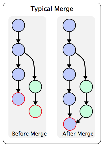
merge: to combine changes on another branch into the current branch

conflict: differences that cannot automatically be merged

headless: HEAD does not point to any branch

Detached HEAD: refers to a situation where the HEAD pointer (which usually points to a branch reference) directly points to a specific commit, rather than pointing to the latest commit of a branch.

In simpler terms, when you’re working in a normal branch (say, “master” or “main”), the HEAD points to the name of that branch, and that branch name points to the latest commit.

Any new commits you make will advance the branch to point to the newer commit, and HEAD follows along because it’s pointing to the branch name.

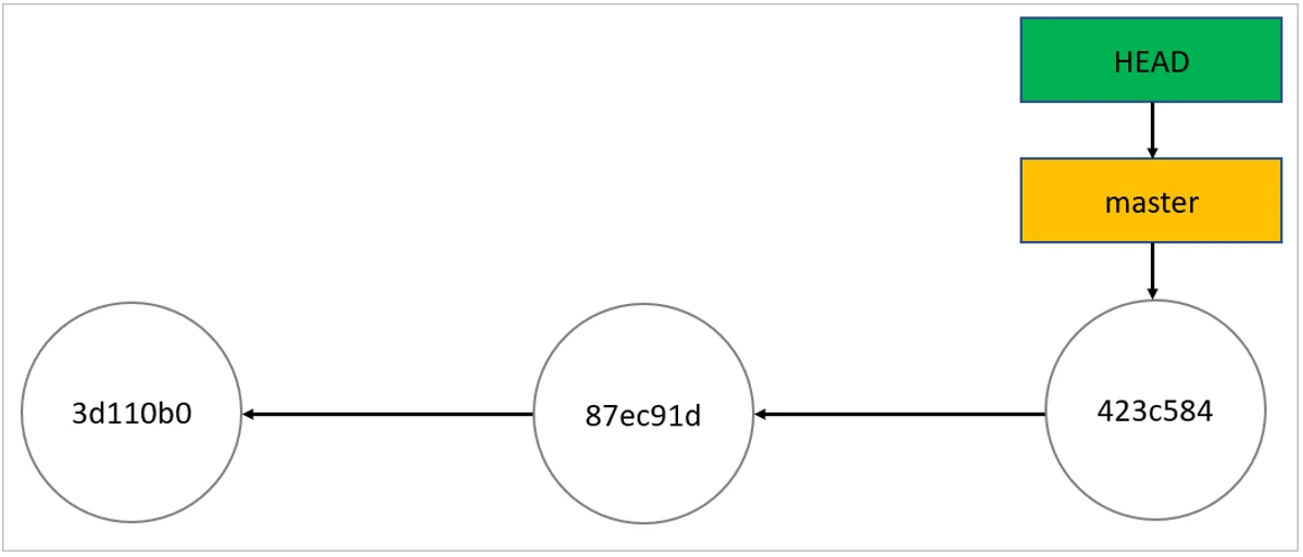
As you can see, HEAD points to the controller branch, which points to the last commit. Everything looks perfect. After running git checkout 87ec91d, the repo looks like this:

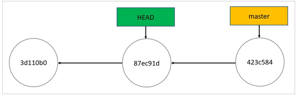
This is the detached HEAD state; HEAD is pointing directly to a commit instead of a branch.

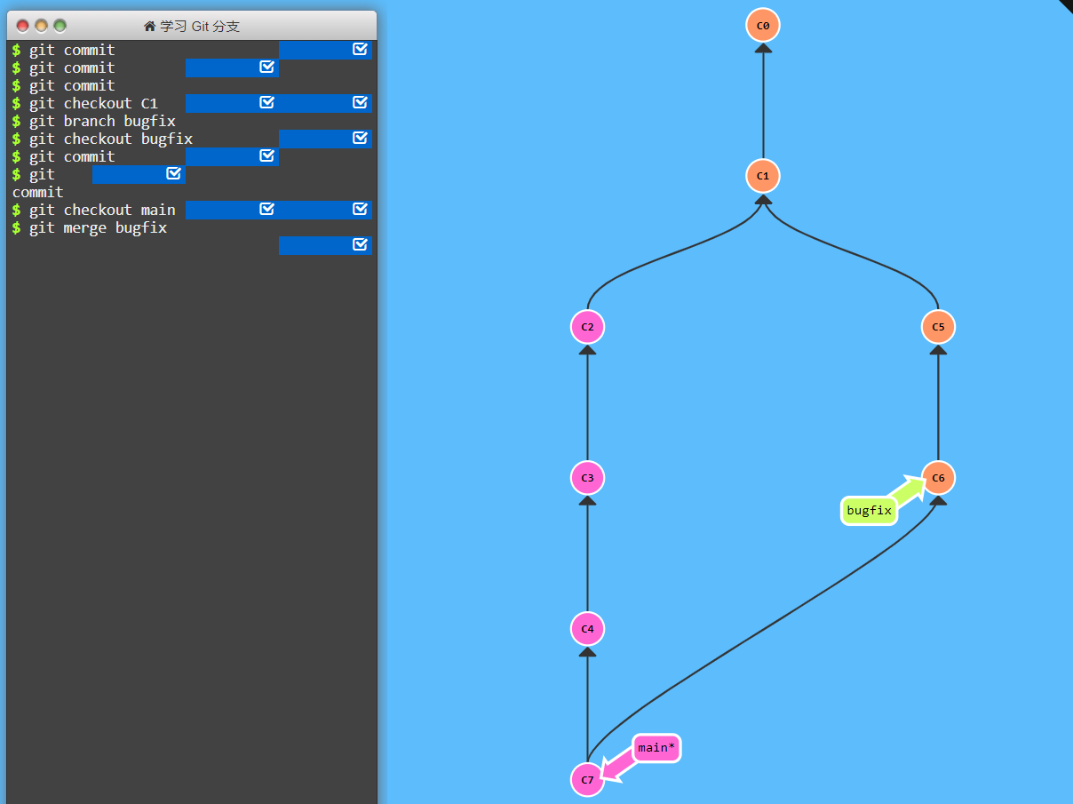
git demonstration

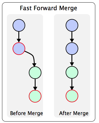
fast forwarding: If master has not diverged, instead of creating a new commit, git will then simply point master to the latest commit of the feature branch. This is a “fast forward”.

如果合并的两个branch在一条线上，git checkout 前面的branch，merge后面的，就会触发fast forwarding

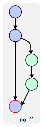
--no--ff means 不用fast forwarding

If you’re on branch x and run ‘git merge y’, then you will point to new branch named x

When making a git commit, the head is recommend to point to branch, otherwise may cause detached HEAD problem

checkout:

• output is bytes, not string

• checkout(["git","commit",cwd="directory_name")

Performance

Things that affect performance:

• speed of the computer (CPU, etc)
• speed of Python (quality+efficiency of interpretation)
• algorithm: strategy for solving the problem
• input size: how much data do we have?

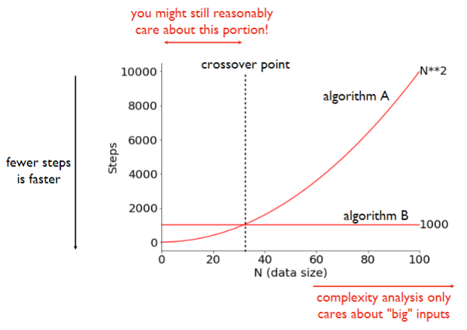
when analyze complexity, only care about big inputs

A step is any unit of work with boudned execution time. (“bounded” does not mean “fixed”)

Big O

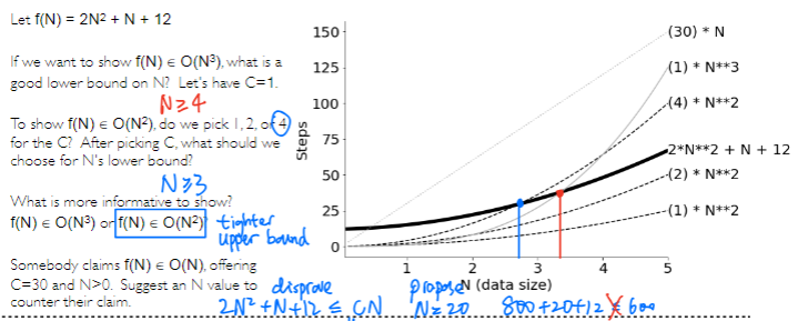
If $f(N) \leq C * g(N)$, then $f(N) \in O(g(N))$

Common complexity for list operation:

• $O(1)$: len(L),L[-1],L[-10],L.append(x),L.pop(-1)

• $O(N)$: L.insert(0,x),L.pop(0),max(L),min(L),sum(L),L2.extend(L1),found x in L

Special case:

for deque(双端队列): $O(1)$deque.popleft(0),deque.pop()

for heapq(小根堆): $O(1ogN)$ heapq.heappop(), heapq.heappush(x)

$O(N)$ heapq.heapify(L)

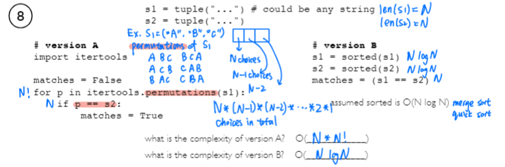
Examples

看图说话

Object Oriented Programming

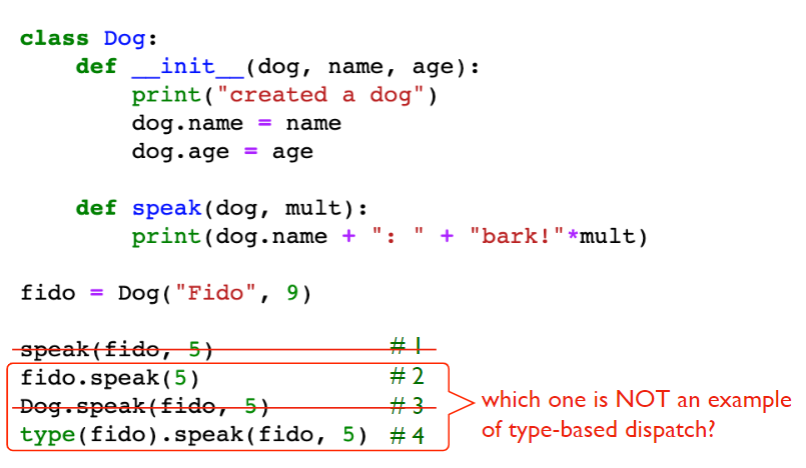
Dog.speak(fido,5)is NOT an example of type-based dispatch

fido.speak(5)is preferred

def __init__(dog,name,age): self is better than dog for the receiver parameter

Special Methods

Not all __some__ is special methods

implicitly called

__str__ vs__repr__

__str__, __repr__, control how an object looks when we print it or see it in Out[N] print(),str()方法会调用到__str__方法，print(),str(),repr()方法会调用__repr__方法。从下面的例子可以看出，当两个方法同时定义时，Python会优先搜索并调用__str__方法。

>>> class Str(object):
...     def __str__(self):
...         return "__str__ called"    
...     def __repr__(self):
...         return "__repr__ called"
... 
>>> s = Str()
>>> print(s)
__str__ called
>>> repr(s)
'__repr__ called'
>>> str(s)
'__str__ called'

__repr__

• The __repr__ method is used to define the “official” string representation of an object. It is used by the repr() built-in function and by backticks (`) in Python 2.x.
• The string returned by __repr__ should be a valid Python expression that, when evaluated, would create an object with the same state as the original object. In other words, it should be unambiguous and precise.
• This method is primarily used for debugging and development purposes.

__str__:

• The __str__ method is used to define the “informal” or “user-friendly” string representation of an object. It is used by the str() built-in function and by the print() function.
• The string returned by __str__ should be readable and understandable to users.
• If __str__ is not defined, the __repr__ method will be used as a fallback.

In summary, __repr__ is more for developers, providing a detailed and unambiguous representation* of an object, while __str__ is for users, presenting a more user-friendly and readable representation of the object. It’s common to implement __repr__ and optionally __str__ for your custom classes to enhance their debuggability and usability.

__repr_html__, generate HTML to create more visual representaitons of objects in Jupyter.

__eq__, __ne__, __lt__, __ge__,__le__, __ge__,define how ==, !=, <, >, <=, >= behaves for two different objects, for sorted, must implement __lt__

__len__, __getitem__, build our own sequences that we index, slice, and loop over.

__enter__, __exit__, context managers, (like automatically close file)

with语句，先调用__enter__在__init__之后，在with结束后调用__exit__

positional arguments includes self

def getgrade(name, score):
    """ This function computes a grade given a score"""
    if score > 80:
        grade = 'A'y
    elif 80 > score > 70:
        grade = 'B'
    elif 70 > score > 60:
        grade = 'C'
    else:
        grade = 'D'

    return name + " had grade: " + grade 
getgrade('prince', 78) # To call this function using positional arguments:
getgrade(name='prince', score=78) # using keyword arguments:  

positional arguments就是不带=，带=就是keyword

Attributes are the individual data items or characteristics associated with an object.

• class attribute

• instance attribute

class MyClass:
    class_attribute = 42  # 'class_attribute' is a class attribute
    def __init__(self, value):
        self.value = value  # 'value' is an instance attribute

obj1 = MyClass(10)

print(obj1.value)  # Out put 10
print(obj1.class_attribute)  # Output: 42

Assume Car is one of the child class of Vehicle. Which of the following allows me to call the drive() method defined in the Vehicle class within the Car class?

• super().drive()

• Vehicle.drive(self)

The X class is a parent of the Y class; both have an __init__method. Both __init__ methods are guaranteed to run when a new instance of Y is created, regardless of the code in Y’s __init__ method.

• False

htop shows how much memory is being used

TextIOWrapper is for converting bytes to str

What is the benefit of reading a CSV inside a .zip file directly from Python, without unzipping it from the command line first?

• to save storage space

What is the benefit of using csv.DictReader instead of pd.read_csv ?

• save memory space

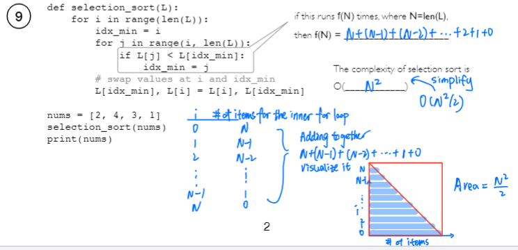
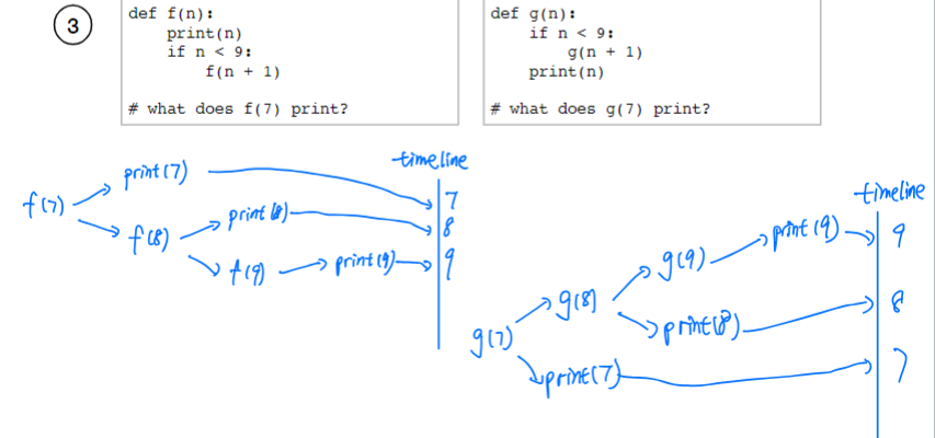
Recursion

Call graph

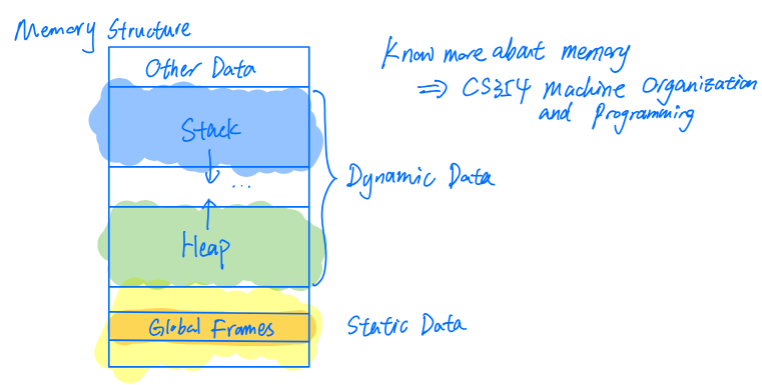
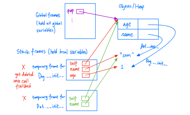
Memory

global frames hold all global variables

stack frames hold local variables

Each function can have multiple frames on the stack at a time.

BST

左儿子比自己小，右儿子比自己大，建树和输入顺序有关系

randomly input 会让树更balanced

insert 复杂度 $O(H)$ 最坏$O(N)$ 最好$O(logN)$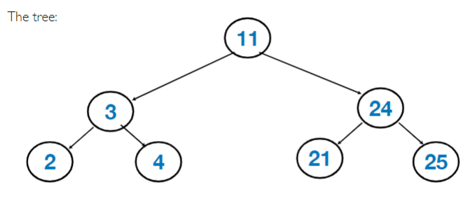

Search

DAG : 有向无环图

Strongly connected: 强连通图，考虑direction，所有节点都能相互走到

Weakly connected：弱联通，忽略方向，所有节点都能互相到达

Acyclic：无环

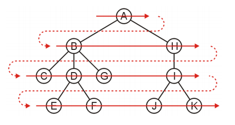
DFS

优先深节点

用stack栈，每次加入节点的孩子，先加大的再小的（保证尾巴先出来的是小的），尾进尾出

对于环，遇到已经加到栈的孩子仍然新加一个相同的

A

H B

H E C

H E D

H E

H G F

H G

H

M I

M L K J

M L

M

A, B, C, D, E, F, G, H, I, J, K, L ,M

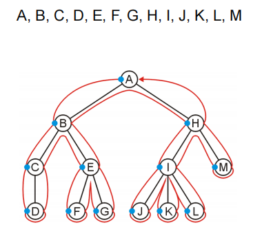
BFS

优先更浅的节点

用deque双端队列，每次加入节点的孩子，先加小的再大的，尾进头出

A

B H

H C D G

C D G I

D G I

G I E F

I E F

E F J K

F J K

J K

K

A, B, H, C, D, G, I, E, F, J, K

Selenium

DOM

Every web page is a tree.

Elements (nodes of the DOM (document object model) tree) may contain attributes, text, and other elements.

JavaScript can directly edit the DOM tree.

Browser renders (displays) DOM tree, based on original HTML (hyper-text markup language) file and any JavaScript changes.

DAG, weakly connected graph is right. Binary tree is false.

Web Scraping

request can fetch html, js, etc file.

Selenium can fetch html, js, etc file, run a js file in browser, and grab HTML version of DOM after JavaScript has modified it.

Finding Elements on Webpages

WebDriver.get(u) loads the web page with URL (uniform resource locator) u

WebDriver.find_element(a, b) returns the first WebElement which has attribute a being b, and

WebDriver.find_elements(a, b) returns a list of WebElements:

Common Attributes

WebDriver.find_element("id", id) locates the element by its unique ID.
WebDriver.find_element("name", id) locates the element by its names, but multiple elements can have the same name.
WebDriver.find_element("tag name", id) locates the element by its tag, some of the common tags include:

Tag	Element	Example
a	hyperlink	Link
button	button	button
code	code	code
div or span	section	span
h1 to h6	headings
img and video	image and video
input and textarea	text fields
ol or ul	ordered or unordered list	li is an item
p	paragraph
select	drop-down list	1/ 2 / 3
table	table	tr is a row, and td is a cell in the table

Tables can be scraped by find_element("tag name", "table") and iterate over find_elements("tag name", "tr") and find_elements("tag name", "td")

pandas.read_html can return a list of DataFrames, one for each table, on the web page.

$j$th cell of first row: element.find_element("tag name", "tr")[i - 1].find_elements("tag name", "td")[j - 1].text

$j$th cell of $i$th row: element.find_elements("tag name", "tr")[i - 1].find_elements("tag name", "td")[j - 1].text

Screenshot

WebDriver.save_screenshot("file.png") saves a screenshot of the web page to a file with name file.png.

Sometimes the screenshot only captures only a part of the page: Firefox has the option to take screenshot of the full page using WebDriver.save_full_screenshot("file.png").

Alternatively, a screenshot of a specific element can be save using WebElement.screenshot("file.png").

Others

WebDriver.find_elements("tag_name", "a") finds all the hyperlinks on the page.

Use url = WebElement.get_attribute("href") to get the URL of the hyperlink, then use WebDriver.get(url) to load that page.

Polling

Use time.sleep(s) to wait s seconds, and use it inside a while loop to wait for an event to happen, before accessing or interacting with the updated elements.

Avoid infinite loops by setting a maximum amount of time to wait.

selenium.webdriver.support has implicit and explicit waits, so that the driver keeps polling until a certain condition is met or a certain time has passed

from selenium import webdriver
from selenium.webdriver.common.by import By
from selenium.webdriver.support.wait import WebDriverWait
from selenium.webdriver.support import expected_conditions as EC

driver = webdriver.Firefox()
driver.get("http://somedomain/url_that_delays_loading")
try:
    element = WebDriverWait(driver, 10).until(
        EC.presence_of_element_located((By.ID, "myDynamicElement"))
        // WebDriver.find_element("id", id)
    )
finally:
    driver.quit()

Interact with Elements

Selenium can interact with elements and update the DOM tree.

WebElement.send_keys(t) enters text t into the element (input and textarea), (更新input或者textarea的内容)

WebElement.clear() clears the text in the element, and WebElement.click() clicks the element (buttons)

Robots Exclusion Protocol

urllib.robotparser can be used to check whether a website allows scraping

RobotFileParser.can_fetch(useragent, url) returns True if the useragent (for example, "*") is allowed to fetch url.

Advancing Graph Search

Infinite Graph Search

If the pages are nodes, and links on one page to another page are edges, the digraph formed by pages will possibly have infinite depth and may contain cycles.

To find a specific (goal) page, or to discover reachable pages from the initial page, breadth first search should be used (since depth first search may not terminate on trees with infinite depth).

Since there are cycles, a list of visited pages should be kept.

Search Heuristics

A search heuristic is an estimate of how close the current node is to the goal node in the search tree.

Before the start of a search, the heuristic functions may not be accurate estimates of the distances from the current node to the goal node.

A heuristic that always underestimates the true distance is called an admissible heuristic.

①admissible：$0\leq h(n)\leq h^*(n)$，小于实际n到终点的距离。

Informed Search

Searching the nodes in the order according to the heuristic is called best first greedy search (GBS, since BFGS is reserved for the non-linear optimization method, Link).

贪心：只考虑H最小

Since the heuristic could be incorrect, it might not find the shortest path to the goal node.

Searching the nodes in the order according to the current distance from the initial node plus the heuristic is called A search (the name of the search algorithm is “A”)

If the heuristic is admissible, A search is called A* search (A-star search).

For GBS search, use a Priority Queue with the priority based on the heuristic Only h

For A search, use a Priority Queue with the priority based on current distance plus the heuristic. h+g

A goal node that is reachable (finite edges away) from the initial node, but the following method cannot find the goal node.Assume the nodes are {G,0,1,2,…} where 0 is the initial node and G is the goal node, and each node has finite number of children.

BFS & A: will find the goal

DFS: 深度优先，会优先最深的 $(0,2)(2,G),(0,1),(1,3),(3,4),(4,5),…$

GBS: 启发函数不好，导致先搜索非goal的子树

Flask

Flask will be used to create or modify web pages. It can be useful for collecting visitor data when interacting with the web pages and displaying them on the web pages

Flask is a simpler web framework of Django. Django is a more popular package.

Basics

app = flask.Flask(...) to create a web app

`@app.route(“/“)` binds a function to the root URL (front page of the website).

`@app.route(“/abc”)` binds a function to a specific URL path on the site (one page on the website, or a file).

app.run(host="0.0.0.0", debug=False, threaded=False) to run the app. host="0.0.0.0" makes the server externally visible.

flask.Response: enables us to create a response object instance

• Arguments: str representing repsonse, headers dict representing metadata, status representing status code.
• flask.request.remote_addr: enables us to take action based on the IP address from which we receive the request
• flask.request.args: enables us to get the arguments passed as part of the URL
  • How do we pass arguments?
    • at the end of the URL, add a “?”
    • then separate argument-value pair by “=”
    • use “&” as delimiter between two argument-value pairs
    • examples:
      • http://34.69.204.31:5000/add?x=10&y=20
      • http://34.69.204.31:5000/survey?major=CS
      • http://34.69.204.31:5000/survey?major=Mechanical Engineering

flask.request.args enables us process query string
`@app.route(““, methods=[“POST”])enables us to process HTTP POST requestsflask.request.get_data()` enables us to access data (byte format) sent via HTTP POST request

Binding a Function to an URL Path

@app.route("/index")
    def index():
    return "Hello World!"

binds the index function to the page IP address/index, meaning it will display a web page that says “Hello World”.

“Hello World” can be replaced by any text or HTML string, which can be read from an HTML file and modified in the index() function.

HTML string can be read from existing HTML files then modified, for example

with open("index.html") as f: return f.read().

It can also be generated by packages such as pandas, for example, pandas.read_csv("data.csv").to_html().

Binding Multiple Paths

@app.route("/index/<x>") 
    def index(x): 
        return f"Hello {x}"

To bind multiple paths, variable rules can be added, will display a web page that says “Hello World” when the path IP address/index/World is used.

The variable x can also be converted to another type for the index(x) function.

Route	Type	Description
`@app.route(“/index/“)`	string	Default
`@app.route(“/index/int:x“)`	int	Convert to Integer
`@app.route(“/index/float:x“)`	float	Convert to Float
`@app.route(“/index/path:x“)`	path	String but allows /

Redirect

return flask.redirect(url) redirects the current path to another with URL url.

return flask.redirect(flask.url_for("index")) redirects the current path to another which binds to the function index().

return flask.redirect(flask.url_for("index", x = "World")) redirects the current path to another which binds to the function index("World").

Collecting Information

flask.request.remote_addr can be used to find the remote IP address of the visitor

IP addresses can be then used to find visitor information such as their service provider, location (country, state, city)

flask.request.user_agent.string can be used to find the user agent of the visitor.

User Agent information can be used to find browser, operating system, device information

The visitors’ IP addresses then can be stored in global variable or saved to a file on the server to keep track of who visited each page and when.

Rate Limiting

One use of such visitor information is for rate limiting: preventing visitors from loading the pages too often, for example, to prevent web scraping.

In this case, the visitor’s IP address and visit time can be stored in a list: in case the next visit time is too close to the previous one, the visitor can be redirected to another page, or more commonly, responded with a error message, for example, return flask.Response("...", status = 429, headers = {"Retry-After": "60"} tells the visitor to retry after 60 seconds.

A list of response status and header fields can be found: here status = 429 says “Too Many Requests”.

requests module:

• resp = requests.get(<URL>) method: enables us to send HTTP GET request
• resp.status_code: status code of the response
• resp.text: str text content of the response
• resp.headers: dict content of response headers

Live Plots on Flask Sites

A function that returns an image response can be used for `@app.route(“/plot.png”)or@app.route(“/plot.svg”)`. (SVG is Scalable Vector Graphics and vector graphics is represented by a list of geometric shapes such as points, lines, curves, PNG is Portable Network Graphics and raster graphics is represented by a matrix of pixel color values)

An image response can be created using flask.Response(image, headers={"Content-Type": "image/png"}) or flask.Response(image, headers={"Content-Type": "image/svg+xml"}), where the image is a bytes object and can be obtained using io.BytesIO.getvalue() where io.BytesIO creates a “fake” file to store the image.

On the web page, display the image as <img src="plot.png"> or <img src="plot.svg">.

AB Testing

Concept

Two or more versions of the same page can be displayed to the visitor randomly to compare which one is better.

The comparison is often based on click-through rates (CTR), which is computed as the number of clicks on a specific link on the page divided by the number of times the page is displayed to the visitor.

CTR is also used for advertisement, computed as the number of clicks on the ad divided by the number of times the ad is shown to the visitor.

Click Through Rate Example

Suppose the number of clicks are summarized in the following table, what are the click through rates, and is A statistically significantly better than B?

Version	click	no click
A	30	60
B	25	75

The CTR for A is $$\frac{30}{30+60}=\frac{1}{3}$$

The CTR for B is $$\frac{25}{25+75}=\frac{1}{4}$$

Determine whether A is better than B:

• scipy.stats.fisher_exact([[30, 60], [25, 75]]).pvalue=0.1075

原假设 A 不如 B

If a 5 percent threshold is used: 0.1075 > 0.05, 否定原假设，A 并不是显著大于B

if a 20 percent threshold is used: 0.1075 < 0.2, 接受原假设 ，A显著好于B

总结： scipy.stats.fisher_exact([[30, 60], [25, 75]]).pvalue，大于threshold，前面不如后面，小于则一定前面好于后面

Two situations when pvalue will be lower than significance threshold

1. Sample size is the same, but skew is very heavy — unlikely to have that by chance ，差距大？

# Scenario 1: 
# Sample size is the same, but skew is very heavy --- 
# unlikely to have that by chance

df = pd.DataFrame({
    "click":    {"A": 50, "B": 75},
    "no-click": {"A": 50, "B": 25}
})
_, pvalue = stats.fisher_exact(df)
pvalue #0.00042033045869994034

2. Sample size is large, but skew is small

# Scenario 2: 
# Sample size is large, but skew is small 

df = pd.DataFrame({
    "click":    {"A": 500, "B": 550},
    "no-click": {"A": 500, "B": 450}
})
_, pvalue = stats.fisher_exact(df)
pvalue # 0.02820356890423392

Displaying Pages

The choice of which page to display can be random, for example, if random.random() < 0.5: return "Version A" else return "Version B".

It can also be displayed in a fixed ordering, for example, suppose count is a global variable to keep track of the number of visitors, then if count % 2 == 0: return "Version A" else return "Version B" count = count + 1 would alternate between the two versions.

This can be done for a fixed number of times, and after that, only the one with higher click-through rate would be displayed to all visitors.

Query Strings

"index?x=1&y=2" is a URL specifying the path "index" with the query string x=1 and y=2.

Use flask.request.args to get a dictionary of key-value pairs of the query string.

To perform AB testing of a page with two versions, both contain a link to index: on version A, the URL can be <a href="index?from=A">Link<\a>, and on version B, the same URL can be <a href="index?from=B">Link<\a>.

If version A URL is used, request.args["from"] would be "A" and if version B URL is used request.args["from"] would be "B".

Multi-Armed Bandit

The previous design has experiments with alternatives for a fixed number of time then exploit the best alternatives.

This design can lead to a large “regret”, for example, if displaying bad version is costly. In other settings such as drug or vaccine trials and stock selection, experimenting with bad alternatives can be costly.

The problem of optimal experimentation vs exploitation is studied in reinforcement learning as the multi-armed bandit problem:

Upper Confidence Bound

Upper Confidence Bound (UCB) is a no-regret algorithm that minimizes the loss from experimentation.

After every version is displayed once, the algorithm keeps track of the average value (for example click-through rate) from each version, say $ \hat{\mu_A},\hat{\mu_B} $, computes the UCBs $\hat{\mu_A} + c \sqrt{ \frac{2 log(n)}{n_A}}$ and $\hat{\mu_B} + c \sqrt{ \frac{2 log(n)}{n_B}}$

where $n$ is the total number of visitors, $n_A$ is the number of visitors of version A, $n_B$ is the number of visitors of version B, and $c$ is a constant, and always picks the version with a higher UCB.

The UCB algorithm uses the principle of optimism under uncertainty and the UCBs are optimistic guesses: with high probability (the probability can be determined by $c$), the actual average is less than UCB.

UCB, choose the highest UCB verison

Visualization

Visual Encodings

Position, size, shape (style), value (light to dark), color (hue), orientation, and texture can be used to present data points in different dimensions. These are called visual encodings.

Some of these encodings are better for different types of features (data dimensions).

Encoding	Continuous	Ordinal	Discrete (Categorical)
Position	Yes	Yes	Yes
Size	Yes	Yes	No
Shape	No	No	Yes
Value	Yes	Yes	No
Color	No	No	Yes
Orientation	Yes	Yes	Yes
Texture	No	No	Yes

Seaborn Plots

seaborn is one of the data visualization libraries that can make plots for exploring the datasets with a few dimensions

Suppose the columns are indexed by c1, c2, …, then seaborn.relplot(data = ..., x = "c1", y = "c2", hue = "c3", size = "c4", style = "c5") visualizes the relationship between the columns by encoding c1 by x-position, c2 by y-position, c3 by color hue if the feature is discrete, and by color value if it is continuous, c4 by size, c5 by shape (for example, o’s and x’s for points, solid and dotted for lines) if the feature is discrete.

Multiple Plots

For discrete dimensions with a small numbers of categories, multiple plots can be made, one for each category.

seaborn.relplot(data = ..., ..., col = "c6", row = "c7") produces multiple columns of plots one for each category of c6, and multiple rows of plots one for each category of c7.

seaborn.pairplot produces a scatter plot for each pair of columns (features) which could be useful for exploring relationships between pairs of continuous features too.

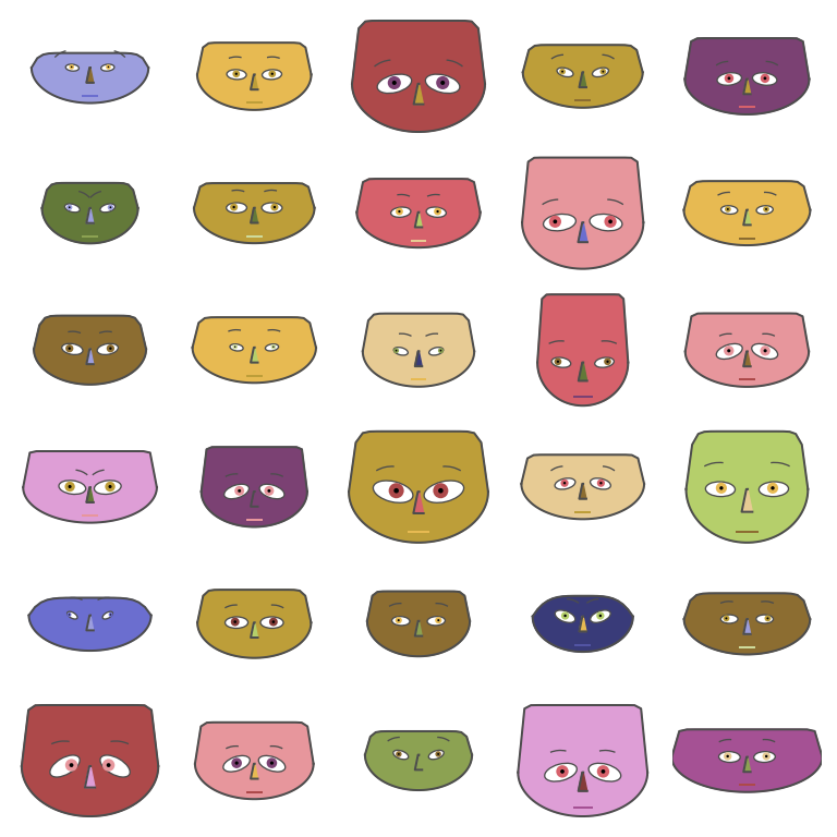
Chernoff Face Example

Chernoff faces can be used to display small low dimensional datasets. The shape, size, placement and orientation of eyes, ears, mouth and nose are visual encodings

ChernoffFace is a package to draw Chernoff Faces

Facial features can be manually designed and plotted in matplotlib.

Plotting High Dimensional Data Sets

If there are large numbers of dimensions and data points, plotting them directly is inappropriate.

To figure out the most important dimensions, which are not necessarily one of the original dimensions, unsupervised machine learning techniques can be used.

One example of such dimensionality reduction algorithms is called Principal Component Analysis (PCA)

Graph

A graph can be represented by node-link lists or adjacency matrices.

To find patterns (for example clusters) in a graph, the positions of the nodes in node-link diagrams or ordering of nodes in adjacency matrices may need to be changed.

Layout

Circular layout and arc (chord) layout are simple for the computer, but difficult for humans to understand the shape of the graph

Force-Directed Placement (FDP) treats nodes as points and edges as springs and tries to minimize energy. It is also called spring model layout

Tree Diagrams

Trees are special graphs for which each node has one parent, and there are more ways to visualize a tree

Many of these visualizations are not available in standard Python plotting packages, but the nodes and edges can plotted “manually” using matplotlib.

Primitives

Custom visualization steps:

• draw “patches” (shapes) on the screen (what):
  • lines
  • polygons
  • circle
  • text
• location of the “patches” on the screen (where):
  • X & Y co-ordinate
  • “Coordinate Reference System (CRS)”:
    • takes some X & Y and maps it on to actual space on screen
    • several CRS

Review: drawing a figure

• fig, ax = plt.subplots(figsize=(<width>, <height>))

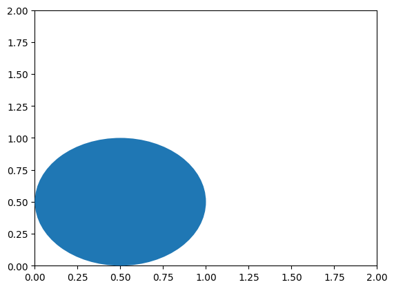
Drawing a circle

• Type plt. and then tab to see a list of patches.
• plt.Circle((<X>, <Y>), <RADIUS>)
• To see the cicle, we need to invoke either:
  • ax.add_patch(<circle object>)
  • ax.add_artist(<circle object>)
  • this invocation needs to be in the same cell as the one that draws the figure
  • Is there a difference between ax.add_patchand ax.add_artist?
    • ax.autoscale_view(): automatically chose limits for the axes; typically works better with ax.add_patch(...)

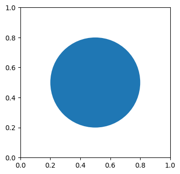
fig, ax = plt.subplots(figsize=(6, 4))
# Let's draw a circle at (0.5, 0.5) of radius 0.3
c = plt.Circle((0.5, 0.5), 0.3)
# type: matplotlib.patches.Circle

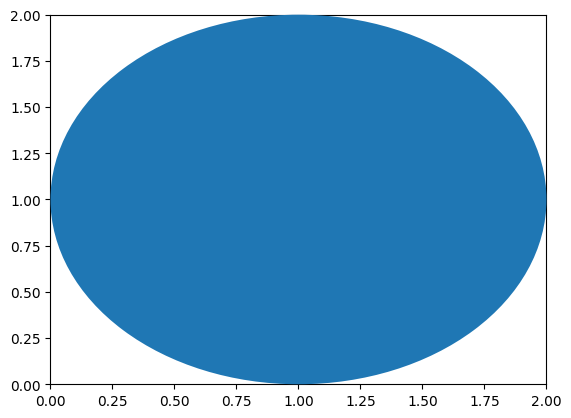
Aspect Ratio

• ax.set_aspect(<Y DIM>): how much space y axes takes with respect to x axes space

fig, ax = plt.subplots(figsize=(6, 4))
c = plt.Circle((0.5, 0.5), 0.3)
ax.add_artist(c)
# Set aspect for y-axis to 1
ax.set_aspect(1)

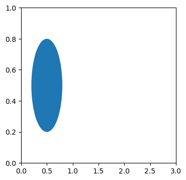
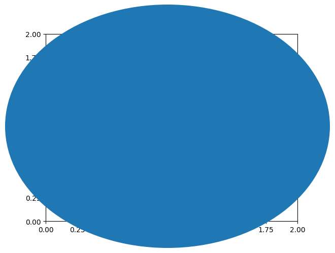
fig, ax = plt.subplots(figsize=(6,4))
# Set x axis limit to (0, 3)
ax.set_xlim(0, 3)
c = plt.Circle((0.5, 0.5), 0.3)
ax.add_artist(c)
# Set aspect for y-axis to 3
ax.set_aspect(3)

matplotlib.patches contain primitive geometries such as Circle, Ellipse, Polygon, Rectangle, RegularPolygon and ConnectionPatch, PathPatch, FancyArrowPatch

matplotlib.text can be used to draw text; it can render math equations using TeX too

A node (indexed i) at ($x,y$) can be represented by a closed shape such as a circle with radius r, for example, matplotlib.patches.Circle((x, y), r), and matplotlib.text(x, y, "i").
➭ An edge from a node at ($x_1,y_1$) to a node at ($x_2,y_2$) can be represented by a path (line or curve, with or without arrow),

Lines: for example, matplotlib.patches.FancyArrowPatch((x1, y1), (x2, y2)), or if the nodes are on different subplots with axes ax[0], ax[1], matplotlib.patches.ConnectionPath((x1, y1), (x2, y2), "data", axesA = ax[0], axesB = ax[1]) 两点连线
➭ To specify the layout of a graph, a list of positions of the nodes are required (sometimes parameters for the curve of the edges need to be specified too).

Curves

A curve (with arrow) from ($x_1,y_1$) to ($x_2,y_2$) can be specified by the (1) out-angle and in-angle, (2) curvature of the curve, (3) Bezier control points

FancyArrowPatch((x1, y1), (x2, y2), connectionstyle=ConnectionStyle.Angle3(angleA = a, angleB = b) plots a quadratic Bezier curve starting from ($x_1,y_1$) going out at an angle a and going in at an angle b to ($x_2,y_2$). 中间控制点$(x_0,y_0)$,angle $\theta_A= arctan(\frac{y_0-y_1}{x_0-x_1})$ $\theta_B= arctan(\frac{y_0-y_2}{x_0-x_2})$
➭ FancyArrowPatch((x1, y1), (x2, y2), connectionstyle=ConnectionStyle.Arc3(rad = r) plots a quadratic Bezier curve from ($x_1,y_1$) to ($x_2,y_2$) that arcs towards a point at distance r times the length of the line from the line connecting ($x_1,y_1$) and ($x_2,y_2$). 中心控制点在两点的垂直平分线上谜案，r代表控制点到中点的距离是两个点距离的几倍

examples:

How to draw a quadratic Bezier curve with control points (0, 0), (1, 0), (1, 1)?
➭ This curve has the same shape as the curve drawn in the “Curve Example”: in particular, the start angle is 0 degrees (measured from the positive x-axis direction) and the end angle is 270 degrees or -90 degrees, and the distance of the line segment connecting the midpoint between (0, 0) and (1, 1) (which is (1/2, 1/2)) and the middle control point (which is (1, 0)) is half of the length of the line segment connecting (0, 0) and (1, 1), or $\sqrt{(1-\frac{1}{2})^2+(0-\frac{1}{2})^2}=\frac{1}{2}\sqrt{(1-0)^2+(1-0)^2}$.
➭ Therefore, use any path patch with connectionstyle ConnectionStyle.Angle3(0, -90) or ConnectionStyle.Arc3(1/2) to plot the curve.

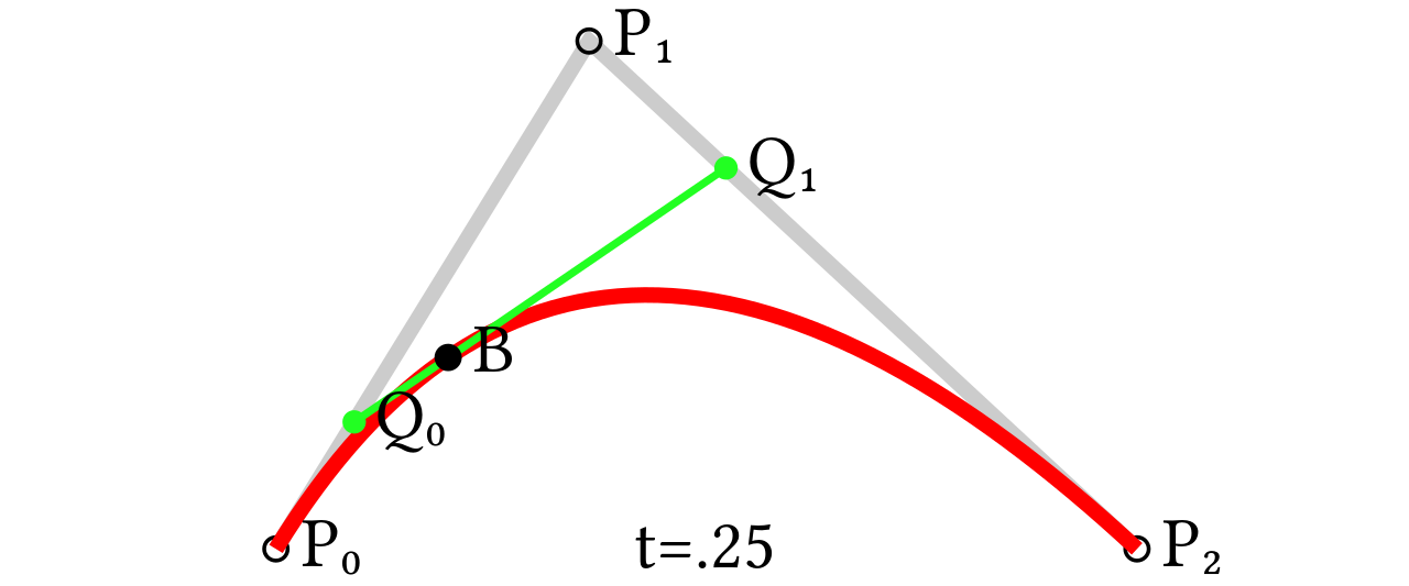
The curves can be constructed by recursively interpolating the line segments between the control points

PathPatch(Path([(x1, y1), (x2, y2), (x3, y3)], [Path.MOVETO, Path.CURVE3, Path.CURVE3])) draws a Bezier curve from ($x_1,y_1$) to ($x_3,y_3$) with a control point ($x_2,y_2$).

PathPatch(Path([(x1, y1), (x2, y2), (x3, y3), (x4, y4)], [Path.MOVETO, Path.CURVE4, Path.CURVE4, Path.CURVE4])) draws a Bezier curve from ($x_1,y_1$) to ($x_4,y_4$) with two control points ($x_2,y_2$) and ($x_3,y_3$).

Coordinate Systems

• fig, ax = plt.subplots(figsize=(<width>, <height>), ncols=<N>, nrows=<N>)

  • ncols: split into vertical sub plots
  • nrows: split into horizontal sub plots

• ax.set_xlim(<lower limit>, <upper limit>): set x-axis limits

• ax.set_ylim(<lower limit>, <upper limit>): set y-axis limits

The primitive geometries can be specified using any of them by specifying the transform argument, for example for a figure fig and axis ax, Circle((x, y), r, transform = ax.transData), Circle((x, y), r, transform = ax.transAxes), Circle((x, y), r, transform = fig.transFigure), or Circle((x, y), r, transform = fig.dpi_scale_trans).

ax.transData

• color parameter controls the color of the “patch”
• edgecolor parameter controls outer border color of the “patch”
• linewidth parameter controls the size of the border of the “patch”
• facecolor parameter controls the filled in color of the “patch”

Coordinate System	Bottom left	Top right	Transform
Data	based on data	based on data	ax.transData (default)
Axes	(0,0)	(1,1)	ax.transAxes
Figure	(0,0)	(1,1)	fig.transFigure
Display	(0,0)	($w,h$) in inches	fig.dpi_scale_trans

(1) ax.transData

(2) ax.transAxes

(3) fig.transFigure

(4) fig.dpi_scale_trans

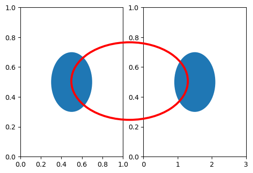
fig, (ax1, ax2) = plt.subplots(ncols=2, figsize=(6, 4))
ax2.set_xlim(0, 3)

# Left subplot
c = plt.Circle((0.5, 0.5), 0.2, transform=ax1.transAxes)
ax1.add_artist(c)

# Right subplot
c = plt.Circle((0.5, 0.5), 0.2, transform=ax2.transAxes)
ax2.add_artist(c)

# whole figure
# edgecolor="red", facecolor="none", linewidth=3
c = plt.Circle((0.5, 0.5), 0.2, transform=fig.transFigure, edgecolor="red", facecolor="none", linewidth=3)
fig.add_artist(c)

No CRS (raw pixel coordinates)

• fig.dpi: dots (aka pixesl) per inch
• increasing dpi makes the figure have higher resolution (helpful when you want to print a large size)
• Review:
  • plt.tight_layout(): avoid unncessary cropping of the figure — always needed for No CRS cases
  • fig.savefig(<relative path.png>): to save a local copy of the image

Map Projections

Positions on a map are usually specified by a longitude and a latitude. It is often used in Geographic Coordinate Systems (GCS).

They are angles in degrees specifying a position on a sphere.

It is difficult to compute areas and distances with angles, so when plotting positions on maps, it is easier to use meters, or Coordinate Reference Systems (CRS).

A region on a map can be represented by one or many polygons.

A polygon is specified by a list of points connected by line segments.

Information about the polygons are stored in shp, shx and dbf files.

GeoPandas

GeoPandas package can read shape files into DataFrames and matplotlib can be used to plot them.

geopandas.read_file(...) can be used to read a zip file containing shp, shx and dbf files, and output a GeoDataFrame, which a pandas DataFrame with a column specifying the geometry of the item.

GeoDataFrame.plot() can be used to plot the polygons.

Conversion from GCS to CRS

GeoDataFrame.crs checks the coordinate system used in the data frame.

GeoDataFrame.to_crs("epsg:326??") or GeoDataFrame.to_crs("epsg:326??) can be used to convert from degree-based coordinate system to meter-based coordinate system.

The ?? in the European Petroleum Survey Group (EPSG) code specifies the Universal Transverse Mercator (UTM) zone
➭ Madison, Wisconsin is in Zone 16.

Polygons

Shapely shapes

Point, LineString, Polygon, MultiPolygon

• from shapely.geometry import Point, Polygon, box

• Polygon([(<x1>, <y1>), (<x2>, <y2>), (<x3>, <y3>), ...]) polygon.Polygon

• box(<x1>, <x2>, <y1>, <y2>) polygon.Polygon

• Point(<x>, <y>) point.Point

• <shapely object>.buffer(<size>)

  • example: Point(5, 5).buffer(3) creates a circle

• Shapely methods:

  • union: any point that is in either shape (OR)
  • intersection: any point that is in both shapes (AND)
  • difference: subtraction
  • intersects: do they overlap?

Creating

Polygons can be created manually from the vertices using shapely too

Point(x, y) creates a point at ($x,y$).

LineString([x1, y1], [x2, y2]) or LineString(Point(x1, y1), Point(x2, y2)) creates a line from ($x_1,y_1$) to ($x_2,y_2$).

Polygon([[x1, y1], [x2, y2], ...]) or Polygon([Point(x1, y1), Point(x2, y2), ...]) creates a polygon connecting the vertices ($x_1,y_1$), ($x_2,y_2$)., …

box(xmin, ymin, xmax, ymax) is another way to create a rectangular Polygon

Properties

Polygon.area or MultiPolygon.area computes the area of the polygon 面积

Polygon.centroid computes the centroid (center) of the polygon 中心

Polygon.buffer(r) computes the geometry containing all points within a r distance from the polygon. 并不是从中心画圆

If Point.buffer(r) is used, the resulting geometry is a circle with radius r around the point, and Point.buffer(r, cap_style = 3) is a square with “radius” r around the point

以中心画一个半径为r的圆

Manipulation

Union and intersections of polygons are still polygons.

geopandas.overlay(x, y, how = "intersection") computes the polygons that is the intersection of polygons x and y, 返回交集

.intersects()返回是否相交

if GeoDataFrame has geometry x, GeoDataFrame.intersection(y) computes the same intersection

GeoDataFrame.difference(y): Returns a GeoSeries of the points in each aligned geometry that are not in other.

.symmetric_difference(): Returns a GeoSeries of the symmetric difference of points in each aligned geometry with other.

geopandas.overlay(x, y, how = "union") computes the polygons that is the union of polygons x and y， if GeoDataFrame has geometry x, GeoDataFrame.union(y) computes the same union

GeoDataFrame.unary_union is the single combined MultiPolygon of all polygons in the data frame

GeoDataFrame.convex_hull computes the convex hull (smallest convex polygon that contains the original polygon)

Convex

A shape is convex if the shape contains the whole line segment between any two points in the shape.

box(0, 0, 1, 1): yes, all rectangles are convex.

Point(0, 0).buffer(1): yes, all circles (or polygon approximations of circles) are convex.

Polygon([[0, 0], [1, 0], [0, 1]]: yes, any triangle is convex.

box(0, 0, 2, 2).intersect(box(1, 1, 3, 3)): yes, the intersection here is just box(1, 1, 2, 2), and in general, the intersection between any two convex shapes is still convex.

box(0, 0, 2, 2).union(box(1, 1, 3, 3)): no, the line segment between (0, 2) and (1, 3) is not inside the shape.

box(0, 0, 2, 2).union(box(1, 1, 3, 3)).convex_hull: yes, the convex hull of any shape is convex.

Point(0, 0).buffer(1).boundary: no, the boundary is a circle without the inside (approximated by a lot of line segments), and the line segment connecting any two distinct points on the circle is not on the boundary, and in general, the boundary of any shape with strictly positive area is not convex.

Geocoding

geopy provide geocoding services to convert a text address into a Point geometry that specifies the longitude and latitude of the location

geopandas.tools.geocode(address) returns a Point object with the coordinate for the address.

Lat / long CRS

• Long is x-coord
• Lat is y-coord
  • tells you where the point on Earth is
• IMPORTANT: degrees are not a unit of distance. 1 degree of longitute near the equator is a lot farther than moving 1 degree of longitute near the north pole

Using .crs to access CRS of a gdf.

Single CRS doesn’t work for the whole earth

• Setting a different CRS for Europe that is based on meters.

Regex

Regular Expressions (Regex) is a small language for describing patterns to search for and it is used in many different programming languages

Python re package has re.findall(regex, string) and re.sub(regex, replace, string) to find and replace parts of string using the pattern regex.

re.findall(regex, string) return a list

Raw Strings

Python uses escape characters to represent special characters.

Raw strings r"..." starts with r and do not convert escape characters into special characters.

It is usually easier to specify regex with raw strings.

Code	Character	Note
\"	double quote	-
\'	single quote	-
\\	backslash 反斜杠	"\\ \" " displays \"
\n	new line	-
\r	carriage return	(not used often)
\t	tab “ “	-
\b	backspace	(similar to left arrow key)

\\ 表示转义\后面的符号，这个就是转义\ = \

Raw String Examples

• "\t" == r" " is true.
• "\\t" == r"\t" is true.
• "\\\t" == r"\ " is true.
• "\\\\t" == r"\\t" is true.
• "A\\B\\C" == r"A\B\C" is true.

Meta Characters

Some characters have special functions in a regex, and they are called meta characters.

Meta character	Meaning	Example	Meaning
.	any character except for \n	-	-
[]	any character inside brackets	[abc]	a or b or c
[^ ]	any character not inside brackets	[^abc]	not one of a b c
*	zero or more of last symbol	a*	zero or more a
+	one or more of last symbol	a+	one or more a
?	zero or one of last symbol	a?	zero or one a
{ }	exact number of last symbol	a{3}	exactly aaa
{ , }	number of last symbol in range	a{1, 3}	a or aa or aaa
`	`	either before or after bar	`ab	bc`	either ab or bc
\	escapes next metacharacter 转义	\?	literal ?
^	beginning of line	^a	begins with a
$	end of line	a$	ends with a

*? 非贪婪匹配，匹配到一个就停止

Shorthand

Some escape characters are used as shorthand.

Shorthand	Meaning	Bracket Form
\d	digit	[0-9]
\D	not digit	[^0-9]
\w	alphanumeric character	[a-zA-Z0-9]
\W	not alphanumeric character	[^a-zA-Z0-9]
\s	white space	[\t\n\r]
\S	not white space	[^\t\n\r]

Capture Group

re.findall can return a list of substrings or list of tuples of substrings using capturing groups inside (...), for example, the regex ...(x)...(y)...(z)... returns a list of tuples with three elements matching x, y, z. using((x),(y)) , return [(xy,x,y)]

re.sub can replaces the matches by another string, the captured groups can be used in the replacement string by \g<1>, \g<2>, \g<3>, …, for example, replace ...(x)...(y)...(z)... by \g<2>\g<3>\g<1> will return yzx.

最外面的括号表示第一个是整体

Data Preprocessing

Feature Representation

Items need to be represented by vector of numbers, item i is $\left(x_{i1}, x_{i2}, …, x_{im}\right)$.

Some features are already represented by real numbers, sometimes need to be rescaled to [0,1].

Some features are categories, could be converted using one-hot encoding.

Images features and text features require additional preprocessing.

Text

Tokenization

A text document needs to be split into words.

Split the string by space and punctuation, sometimes regular expression rules can be used.

Remove stop words: “the”, “of”, “a”, “with”, …

Stemming and lemmatization: “looks”, “looked”, “looking” to “look”.

nltk has functions to do these. For example, nltk.corpus.stopwords.words("english") to get a list of stop words in English, and nltk.stem.WordNetLemmatizer().lemmatize(word) to lemmatize the token word.

Vocabulary

A word token is an occurrence of a word.

A word type is a unique word as a dictionary entry.

A vocabulary is a list of word types, typically 10000 or more word types. Sometimes <s> (start of sentence), </s> (end of sentence), and <unk> (out of vocabulary words) are included in the vocabulary.

A corpus is a larger collection of text (like a DataFrame).

A document is a unit of text item (like a row in a DataFrame).

Bag of Words Features

sklearn.feature_extraction.text.CountVectorizer can be used to convert text documents to a bag of words matrix

sklearn.feature_extraction.text.TfidfVectorizer can be used to convert text documents to a bag of words matrix

Bag of words features represent documents as an unordered collection of words.

Each document is represented by a row containing the number of occurrences of each word type in the vocabulary.

For word type j and document i, the feature is $c\left(i, j\right)$ the number of times word j appears in document i.

TF-IDF Features

TF-IDF or Term Frequency Inverse Document Frequency features adjust for the fact that some words appear more frequently in all documents

The term frequency of word type j in document i is defined as $\text{tf} \left(i, j\right) = \dfrac{c\left(i, j\right)}{\displaystyle\sum_{j’} c\left(i, j’\right)}$ where $c\left(i, j\right)$ is the number of times word j appears in document i, and $\displaystyle\sum_{j’} c\left(i, j’\right)$ is the total number of words in document i.

The inverse document frequency of word type j in document i is defined as $\text{idf} \left(i, j\right) = \log \left(\dfrac{n + 1}{n\left(j\right) + 1}\right)$ where $n\left(j\right)$ is the number of documents containing word j, and n is the total number of documents.

For word type j and document i, the feature is $\text{tf} \left(i, j\right) \cdot \text{idf} \left(i, j\right)$.

Images

Image Pixel Intensity Features

Gray scale images have pixels valued from 0 to 255 (integers, 0 being black, 255 being white), or from 0 to 1 (real values, 0 being black, 1 being white).

These pixel values are called pixel intensities.

The pixel value matrices can be flattened into a vector (i.e. k pixel by k pixel image can be written as a list of k^2 numbers and used as input features.

scikit-image can be used for basic image processing tasks

skimage.io.imread (read image from file), skimage.io.imshow (show image)

The images are stored as numpy.array, which can be flattened using numpy.ndarray.flatten

Color Images

RGB color images have color pixels represented by three numbers Red, Green, Blue, each valued from 0 to 255 or 0 to 1.

Intensity can be computed as $I = \dfrac{1}{3} \left(R + G + B\right)$.

Other perceptual luminance-preserving conversion can be done too, for example $I = 0.2125 R + 0.7154 G + 0.0721 B$.

skimage.color.rgb2gray (convert into gray-scale)

The pixel value 3D arrays can be converted into pixel intensity matrices and flattened into a feature vector.

Convolution

Convolution between an image and a filter (sometimes called kernel) is the dot product of every region of an image and the filter (sometimes flipped).

Convolution with special filters detects special features.

skimage.filters has a list of special filters

Name	Example	Use
Identity	$\begin{bmatrix} 0 & 0 & 0 \ 0 & 1 & 0 \ 0 & 0 & 0 \end{bmatrix}$	nothing
Gaussian	$\begin{bmatrix} 0.0625 & 0.125 & 0.0625 \ 0.125 & 0.25 & 0.125 \ 0.0625 & 0.125 & 0.0625 \end{bmatrix}$	blur
X gradient	$\begin{bmatrix} 0 & 0 & 0 \ 1 & 0 & -1 \ 0 & 0 & 0 \end{bmatrix}$	vertical edges
Left (Right) Sobel	$\begin{bmatrix} 1 & 0 & -1 \ 2 & 0 & -2 \ 1 & 0 & -1 \end{bmatrix}$	vertical edges (blurred)
Y gradient	$\begin{bmatrix} 0 & 1 & 0 \ 0 & 0 & 0 \ 0 & -1 & 0 \end{bmatrix}$	vertical edges
Top (Bottom) Sobel	$\begin{bmatrix} 1 & 2 & 1 \ 0 & 0 & 0 \ -1 & -2 & -1 \end{bmatrix}$	vertical edges (blurred)

Supervised Learning

Supervised learning (data is labeled): use the data to figure out the relationship between the features and labels of the items, and apply the relationship to predict the label of a new item.

If the labels are discrete (categories): classification.

If the labels are continuous: regression.

Binary Classification

For binary classification, the labels are binary, either 0 or 1, but the output of the classifier $\hat{f}(x)$ can be a number between 0 and 1.

$\hat{f}(x)$ usually represents the probability that the label is 1, and it is sometimes called the activation value.

If a deterministic prediction $\hat{y}$ is required, it is usually set to $\hat{y}=0$ if $\hat{f}(x) \leq 0.5 $and $\hat{y}=1$ if $\hat{f}(x) \gt 0.5 $.

Item	Input (Features)	Output (Labels)	-
1	$(x_{11},x_{12},…,x_{1m})$	$y_1∈{0,1}$	training data
2	$(x_{21},x_{22},…,x_{2m})$	$y_2∈{0,1}$	-
3	$(x_{31},x_{32},…,x_{3m})$	$y_3∈{0,1}$	-
…	…	…	…
n	$(x_{n1},x_{n2},…,x_{nm})$	$y_n∈{0,1}$	used to figure out $y \approx \hat{f}(x)$
new	$(x_1’,x_2’,…,x_m’)$	$y’ \in [0,1]$	guess $y’=1$ with probability $\hat{f}(x)$

Confusion Matrix

(1) number of item labeled 1 and predicted to be 1 (true positive: TP),
(2) number of item labeled 1 and predicted to be 0 (false negative: FN),
(3) number of item labeled 0 and predicted to be 1 (false positive: FP),
(4) number of item labeled 0 and predicted to be 0 (true negative: TN).

Count	Predict 1	Predict 0
Label 1	TP	FN
Label 0	FP	TN

Precision is the positive predictive value, or $\frac{TP}{TP+FP}$.
➭ Recall is the true positive rate, or $\frac{TP}{TP+FN}$.
➭ F-measure (or F1 score) is $2·\frac{pr}{p+r} $, where p is the precision and r is the recall

Multi-class Classification

Multi-class classification is different from regression since the classes are not ordered.

Three approaches are used:
(1) Directly predict the probability of each class.
(2) One-vs-one classifiers.
(3) One-vs-all (One-vs-rest) classifiers.

Class Probabilities

If there are k classes, the classifier could output k numbers between 0 and 1, and sum up to 1, to represent the probability that the item belongs to each class, sometimes called activation values.

If a deterministic prediction is required, the classifier can predict the label with the largest probability.

One-vs-one Classifiers

If there are j classes, then $1/2k(k-1)$ binary classifiers will be trained, 1 vs 2, 1 vs 3, 2 vs 3, …

The prediction can be the label that receives the largest number of votes from the one-vs-one binary classifiers.

One-vs-all Classifiers

If there are k classes, then k binary classifiers will be trained, 1 vs not 1, 2 vs not 2, 3 vs not 3, …

The prediction can be the label that achieves the largest probability in the one-vs-all binary classifiers.

Multi-class Confusion Matrix

前面的是行，后面是列

precision of class i is $\frac{c_{ii}}{\sum_j c_{ji}}$(列相同), and recall of class i is $\frac{c_{ii}}{\sum_j c_{ij}}$(行相同).

Conversion from Probabilities to Predictions

Probability predictions are given in a matrix, where row i is the probability prediction for item i, and column j is the predicted probability that item i has label j.

argmax返回index！！！！！！

Given an n×m probability prediction matrix p, p.max(axis = 1) computes the n×1 vector of maximum probabilities, one for each row, and p.argmax(axis = 1) computes the column indices of those maximum probabilities, which also corresponds to the predicted labels of the items.

For example, if p is $\begin{bmatrix} 0.1 & 0.2 & 0.7 \ 0.8 & 0.1 & 0.1 \ 0.4 & 0.5 & 0.1 \ \end{bmatrix}$ , then p.max(axis = 1) is $\begin{bmatrix} 0.7 \ 0.8 \ 0.5\ \end{bmatrix}$ and p.argmax(axis = 1) is $\begin{bmatrix} 2 \ 0 \ 1 \ \end{bmatrix}$

Note: p.max(axis = 0) and p.argmax(axis = 0) would compute max and argmax along the columns.

ps: Pixel intensity usually uses the convention that 0 means black and 1 means white, as done in matplotlib.imshow and skimage.imshow, unlike the example from the previous lecture.

Linear Classifiers

A classifier is linear if the decision boundary is linear (line in 2D, plane in 3D, hyperplane in higher dimensions).

Points above the plane (in the direction of the normal of the plane) are predicted as 1, and points below the plane are predicted as 0.

A set of linear coefficients, usually estimated based on the training data, called weights, $w_1,w_2,…,w_m$, and a bias term b, so that the classifier can be written in the form $\hat{y}=1$ if $w_1x_1’+w_2x_2’+…+w_mx_n’+b \geq 0$ and $\hat{y}=0$ if $w_1x_1’+w_2x_2’+…+w_mx_n’+b <0$

• Linear threshold unit (LTU) perceptron: $g(z)=1$ if $z>0$ and $g(z)=0$ otherwise.
• Logistic regression: $g(z)=\frac{1}{1+e^{-z}}$
• Support vector machine (SVM): $g(z)=1$ if $z>0$ and $g(z)=0$ otherwise, but with a different method to find the weights (that maximizes the separation between the two classes).

Nearest neighbors and decision trees have piecewise linear decision boundaries and is usually not considered linear classifiers.

Note: Naive Bayes classifiers are not always linear under general distribution assumptions.

Activation Function

Sometimes, if a probabilistic prediction is needed, $\hat{f}(x’)=g(w_1x_1’+w_2x_2’+…+w_mx_m’+b)$ outputs a number between 0 and 1, and the classifier can be written in the form $\hat{y}=1$ if $\hat{f}(x’) \geq 0.5$ and $\hat{y}=0$ if $\hat{f}(x’) < 0.5$ .

The function $g$ can be any non-linear function, the resulting classifier is still linear.

Logistic Regression

Logistic regression is usually used for classification, not regression.

The function $g(z)=\frac{1}{1+e^{-z}}$ is called the logistic activation function (or sigmoid function). (z can use $x‘@w+b$)

How well the weights fit the training data is measured by a loss (or cost) function, which is the sum over the loss from each training item $C(w)=C_1(w)+C_2(w)+…+C_n(w)$, and for logistic regression, $C_i(w)=-y_ilog{g(z_i)}-(1-y_i)log(1-g(z_i)),z_i=w_1x_{i1}+w_2x_{i2}+…+w_mx_{im}+b$, called the cross-entropy loss

x@y：矩阵乘法

Classifier的predict都需要一个不等式来划分不同的class

Interpretation of Coefficients

The weight $w_j$ in front of feature j can be interpreted as the increase in the log-odds of the label y being 1, associated with the increase of 1 unit in $x_j$, holding all other variables constant.

This means, if the feature $x_j’$ increases by 1, then the odds of y being 1 is increased by $e^{w_j}$.

The bias b is the log-odds of y being 1, when $x_1’=x_2’=…=x_m’=0$.

Nonlinear Classifiers

Non-linear classifiers are classifiers with non-linear decision boundaries.

Non-linear models are difficult to estimate directly in general.

Two ways of creating non-linear classifiers are,
(1) Non-linear transformations of the features (for example, kernel support vector machine)
(2) Combining multiple copies of linear classifiers (for example, neural network, decision tree)

Sklearn

New features can be constructed manually, or through using transformers provided by sklearn in a sklearn.Pipeline.

A categorical column can be converted to multiple columns using sklearn.preprocessing.OneHotEncoder

OneHotEncoder: Used for categorical variables with discrete values. It converts categorical variables into a binary vector representation, which is not applicable to numerical columns.

(OneHotEncoder(), ["c1"] applied to the categorical column c1 : x cols -> x cols

A numerical column can normalized to center at 0 with variance 1 using sklearn.preprocessing.StandardScaler

StandardScaler is used to scale numerical features to have mean 0 and variance 1, which helps in standardizing the numerical features. Logistic Regression, like many other machine learning algorithms, can benefit from having features on the same scale as it aids in convergence and prevents certain features from dominating due to their larger magnitudes.

Additional columns including powers of one column can be added using (sklearn.preprocessing.PolynomialFeatures,["c2"])

PolynomialFeatures: This is used to create higher-degree polynomial combinations of input features. While it might be useful in some cases to capture nonlinear relationships in data

PolynomialFeatures(degree=2, include_bias=False) applied to the numerical column c2

怎么算根据cols数量确定变量个数 如2 cols = a,b, degree jueding 次方数，逐渐累计，算有多少种组合方式

include_bias=TURE 就+1

Bag of words features can TF-IDF features can be added using feature_extraction.text.CountVectorizer and feature_extraction.text.TfidfVectorizer.

Kernel Trick

sklearn.svm.SVC can be used to train kernel SVMs, possibly infinite number of new features, efficiently through dual optimization (more detail about this in the Linear Programming lecture)

Available kernel functions include: linear (no new features), polynomial (degree d polynomial features), rbf (Radial Basis Function, infinite number of new features).

Neural Network

Neural networks (also called multilayer perceptron) can be viewed as multiple layers of logistic regressions (or perceptrons with other activation functions).

The outputs of the previous layers are used as the inputs in the next layer.

The layers in between the inputs x and output y are hidden layers and can be viewed as additional internal features generated by the neural network.

sklearn.neural_network.MLPClassifier can be used to train fully connect neural networks without convolutional layers or transformer modules. The activation functions logistic, tanh, and relu can be used

PyTorch is a popular package for training more general neural networks with special layers and modules, and with custom activation functions:

Model Selection

Many non-linear classifiers can overfit the training data perfectly

Comparing prediction accuracy of these classifiers on the training set is not meaningful.

Cross validation can be used to compare and select classifiers with different parameters, for example, the neural network architecture, activation functions, or other training parameters.

The dataset is split into K subsets, called K folds, and each fold is used as the test set while the remaining K - 1 folds are used to train.

The average accuracy from the K folds can be used as a measure of the classification accuracy on the training set.

If $k=n$, then there is only one item in each fold, and the cross validation procedure in this case is called Leave-One-Out Cross Validation (LOOCV).

Cross Validation: compare a neural network with two hidden layers and an RBF kernel SVM on a simple 2D dataset using cross validation accuracy.

In a neural network with 4 input features, 3 units in the first hidden layer, 2 units in the second hidden layer, and 1 unit for binary classification in the output layer, how many weights and biases does the network have?

Suppose the activation functions are logistic (other activation functions do not change the answer to this questions), then:
(1) In the first layer, there are 3 logistic regressions with 4 features, meaning there are 12 weights and 3 biases.
(2) In the second layer, there are 2 logistic regressions with 3 features (3 units from the previous layer), meaning there are 6 weights and 2 biases.
(3) In the last layer, there is 1 logistic regression with 2 features (2 units from the previous layer), meaning there are 2 weights and 1 bias.

Therefore, there are 12 + 6 + 1 = 19 weights and 3 + 2 + 1 = 6 biases in the network.

Weights:

• Between Input and First Hidden Layer: Number of weights = (number of input features) * (number of neurons in the first hidden layer)
• Between First Hidden and Second Hidden Layer: Number of weights = (number of neurons in the first hidden layer) * (number of neurons in the second hidden layer)
• Between Second Hidden Layer and Output Layer: Number of weights = (number of neurons in the second hidden layer) * (number of output neurons)

Biases: One bias term is associated with each neuron in the hidden layers and the output layer, except for the input layer which doesn’t have biases.

Linear Algebra

Least Squares Regression

If the label y is continuous, it can still be predicted using $\hat{f}(x’)=w_1x_1’+w_2x_2’+…+w_mx_m’+b$.

scipy.linalg.lstsq(x, y) can be used to find the weights w and the bias n

It computes the least-squares solution to $Xw=y$, or the w such that $||y-Xw||=\sum_{i=1}^n(y_i-w_1x_{i1}-w_2x_{i2}-…-w_mx_{im}-b)^2$ is minimized.

sklearn.linear_model.LinearRegression performs the same linear regression.

Design Matrix

$X$ is a matrix with n rows and m+1 columns, called the design matrix, where each row of $X$ is a list of features of a training item plus a 1 at the end, meaning row i of $X$ is $(x_{i1},x_{i2},…,x_{im},1)$.

The transpose of $X$ , denoted by $X^T$ , flips the matrix over its diagonal, which means each column of $X^T$ is a training item with a 1 at the bottom.

Matrix Inversion

$Xw=y$ can be solved using $w=y/X$ (not proper notation) or $w=X^{-1}y$ only if $X$ is square and invertible.

$X$ has n rows and m columns so it is usually not square and thus not invertible.

$X^tX$ as M+1 rows and M+1 columns and is invertible if $X$ has linearly independent columns (the features are not linearly related)

$X^TXw=X^Ty$ is used, which can be solved as $w=(X^TX)^{-1}(X^Ty)$.

scipy.linalg.inv(A) can be used to compute the inverse of A

scipy.linalg.solve(A, b) can be used to solve for $w$ in $Aw=b$ and is faster than computing the inverse

To solve $Aw=b$, $Aw=c$ for square invertible $A$

Method	Procedure	Speed comparison
1	inv(A) @ b then inv(A) @ c	Slow
2	solve(A, b) then solve(A, c)	Fast
3	lu, p = lu_factor(A) then lu_solve((lu, p), b) then lu_solve((lu, p), c)	Faster

When $A=X^TX$ and $b=X^Ty$, solving $Aw=b$ leads to the solution to the linear regression problem. If the same features are used to make predictions for different prediction variables, it is faster to use lu_solve.

Numerical Instability

Division by a small number close to 0 may lead to inaccurate answers.

Inverting or solving a matrix close to 0 could lead to inaccurate solutions too.

A matrix being close to 0 is usually defined by its condition number, not determinant.

numpy.linalg.cond can be used find the condition number

Larger condition number means the solution can more inaccurate.

Multicollinearity

In linear regression, large condition number of the design matrix is related to multicollinearity.

Multicollinearity occurs when multiple features are highly linearly correlated.

One simple rule of thumb is that the regression has multicollinearity if the condition number of larger than 30.

Regression

Loss Function and R Squared

R squared, or coefficient of determination, $R^2$ is the fraction of the variation of y that can be explained by the variation of x.

The formula for computing R squared is: $R^{2} = 1 - \dfrac{\displaystyle\sum_{i=1}^{n} \left(y_{i} - \hat{y}{i}\right)^{2}}{\displaystyle\sum{i=1}^{n} \left(y_{i} - \overline{y}\right)^{2}}$ or $R^{2} = 1 - \dfrac{\displaystyle\sum_{i=1}^{n} \left(y_{i} - \hat{y}{i}\right)^{2}}{\displaystyle\sum{i=1}^{n} \left(y_{i} - \overline{y}\right)^{2}}$ where $y_i$ is the true value of the output (label) of item $i,\hat{y_i}$ is the predicted value, and $\overline{y}$ is the average value.

Since R squared increase as the number of features increase, it is not a good measure of fitness, and sometimes adjusted R squared is used: $\overline{R}^{2} = 1 - \left(1 - R^{2}\right) \dfrac{n - 1}{n - m - 1}$

R 范围：$[-\inf , 1]$

If model is a sklearn.linear_model.LinearRegression, then model.score(x, y) will compute the $R^2$ on the training set x,y.

Continuous Features

If a feature is continuous, then l in the output if the feature changes by 1 unit, holding every other feature constant.

Similar to the kernel trick and polynomial features for classification, polynomial features can be added using sklearn.preprocessing.PolynomialFeatures(degree = n). Note that the interaction terms are added as well, for example, if there are two columns $x_{1}, x_{2}$, then the columns that will be added when degree = 2 are $1, x_{1}, x_{2}, x_{1}^{2}, x_{2}^{2}, x_{1} x_{2}$

Discrete Features

Discrete features are converted using one hot encoding.

One of the categories should be treated as the base category, since if all categories are included, the design matrix will not be invertible: sklearn.preprocessing.OneHotEncoder(drop = "first") could be used to add the one hot encoding columns excluding the first category.

The weight (coefficient) of $1_{x_{j} = k}$ represents the expected change in the output if the feature j is in the category k instead of the base class.

Log Transforms of Features

Log transformations can be used on the features too.

The weight (coefficient) of $\log\left(x_{j}\right)$ represents the expected change in the output if the feature is increased by 1 percent.

If $\log\left(y\right)$ is used in place of y, then weights represent the percentage change in y due to a change in the feature.

Optimization

Gradient

Loss Minimization

Logistic regression, neural network, and linear regression compute the best weights and biases by solving an optimization problem: $\displaystyle\min_{w,b} C\left(w, b\right)$ where C is the loss (cost) function that measures the amount of error the model is making.

The search strategy is to start with a random set of weights and biases and iteratively move to another set of weights and biases with a lower loss.

Nelder Mead

Nelder Mead method (downhill simplex method) is a derivative-free method that only requires the knowledge of the objective function, and not its derivatives.

Start with a random simplex: a line in 1D, a triangle in 2D, a tetrahedron (triangular pyramid) in 3D, …, a polytope with n+1 vertices in nD.

In every iteration, replace the worst point (the one with the largest loss among the n+1 vertices), by its reflection through the centriod of the remaining n points.

If the new point is better than the original point, expand the simplex; if the new point is worse than the original point, shrink the simplex.

Derivatives

For a single-variable function $C\left(w\right)$, if the derivative at $C’\left(w\right)$, is positive then decreasing w would decrease $C\left(w\right)$, and if the derivative at w is negative then increasing w would decrease $C\left(w\right)$.

In general, $w = w - \alpha C’\left(w\right)$ would update w to decrease $C(w)$ by the largest amount.

Gradient

If there are more than one features, the vector of derivatives, one for each weight, is called the gradient vector, denoted by $\begin{bmatrix} \dfrac{\partial C}{\partial w_{1}} \ \dfrac{\partial C}{\partial w_{2}} \ … \ \dfrac{\partial C}{\partial w_{m}} \end{bmatrix}$ pronounced as “the gradient of C with respect to w” or “D w C” (not “Delta w C”).

The gradient vector represent rate and direction of the fastest change.

$w = w - \alpha \nabla_{w} C$ is called gradient descent and would update w to decrease $C\left(w\right)$ by the largest amount.

The $\alpha$ in $w = w - \alpha \nabla_{w} C$ is called the learning rate and determines how large each gradient descent step will be.
➭ The learning rate can be constant, for example, $\alpha$=1, $\alpha$=0.1, or $\alpha$=0.01; or decreasing, $\alpha = \dfrac{1}{t}$ , $\alpha = \dfrac{0.1}{t}$, or $\alpha = \dfrac{1}{\sqrt{t}}$ in iteration t, and they can be adaptive based on the gradient of previous iterations or the second derivative (Newton’s method).

Newton’s Method

$\nabla^{2}{w} C =\begin{bmatrix} \dfrac{\partial^2 C}{\partial w{1}^2} & \dfrac{\partial C}{\partial w_{1} \partial w_{2}} & … & \dfrac{\partial C}{\partial w_{1} \partial w_{m}} \ \dfrac{\partial C}{\partial w_{2} \partial w_{1}} & \dfrac{\partial^2 C}{\partial w_{2}^2} & … & \dfrac{\partial C}{\partial w_{2} \partial w_{m}} \ … & … & … & … \ \dfrac{\partial C}{\partial w_{m} \partial w_{1}} & \dfrac{\partial C}{\partial w_{m}} \left(w_{2}\right) & … & \dfrac{\partial^2 C}{\partial w_{m}^2} \end{bmatrix}$

It can be used compute the step size adaptively, but it is usually too costly to compute and invert the Hessian matrix.

Newton’s method use the iterative update formula: $w = w - \alpha \left[\nabla^{2}{w} C\right]^{-1} \nabla{w} C$.

Broyden–Fletcher–Goldfarb–Shanno (BFGS) Method

To avoid computing and approximating the Hessian matrix, BFGS uses gradient from the previous step to approximate the inverse of the Hessian, and perform line search to find the step size.

This method is a quasi-Newton method, and does not require specifying the Hessian matrix.

Scipy Optimization Function

scipy.optimize.minimize(f, x0) minimizes the function f with initial guess x0, and the methods include derivative-free methods such as Nelder-Mead, gradient methods such as BFGS (need to specify the gradient as the jac parameter, Jacobian matrix whose rows are gradient vectors), and methods that use Hessian such as Newton-CG (CG stands for conjugate gradient, a way to approximately compute $\left[\nabla^{2}{w} C\right]^{-1} \nabla{w} C$, need to specify the Hessian matrix as the hess parameter).

maxiter specifies the maximum number of iterations to perform and displays a message when the optimization does not converge when maxiter is reached.

tol specifies when the optimization is considered converged, usually it means either the difference between the function (loss) values between two consecutive iterations is less than tol, or the distance between the argument (weights) is less than tol.

Local Minima

Gradient methods may get stuck at a local minimum, where the gradient at the point is 0, but the point is not the (global) minimum of the function.

Multiple random initial points may be used to find multiple local minima, and they can be compared to find the best one.

If a function is convex, then the only local minimum is the global minimum.

The reason cross-entropy loss is used for logistic regression to measure the error is because the resulting $C\left(w\right)$ is convex and differentiable, thus easy to minimize using gradient methods.

Linear Programming 线性规划

A linear program is an optimization problem in which the objective is linear and the constraints are linear.

The set of feasible solutions are the ones that satisfy the constraints, but may or may not be optimal.

The feasible solutions of linear programs form a convex polytope (line segment in 1D, convex polygon in 2D).

Standard Form

The standard form of a linear program is: $ \displaystyle\max_{x} c^\top x$ subject to $A x \leq b$ and $x \geq 0$.
For example, if there are two variables and two constraints, then the standard form is: $\displaystyle\max_{x_{1}, x_{2}} c_{1} x_{1} + c_{2} x_{2}$ subject to $A_{21} x_{1} + A_{22} x_{2} \leq b_{2}$ and $x_{1}, x_{2} \geq 0$, which in matrix form, it is $\displaystyle\max_{\begin{bmatrix} x_{1} \ x_{2} \end{bmatrix}} \begin{bmatrix} c_{1} & c_{2} \end{bmatrix} \begin{bmatrix} x_{1} \ x_{2} \end{bmatrix}$ subject to $\begin{bmatrix} A_{11} & A_{12} \ A_{21} & A_{22} \end{bmatrix} \begin{bmatrix} x_{1} \ x_{2} \end{bmatrix} \leq \begin{bmatrix} b_{1} \ b_{2} \end{bmatrix}$ and $\begin{bmatrix} x_{1} \ x_{2} \end{bmatrix} \geq \begin{bmatrix} 0 \ 0 \end{bmatrix}$.

Dual Form 对偶

The dual form of a linear program in standard form is: $\displaystyle\min b^\top y$ subject to $A^\top y \geq c$ and $y \geq 0$.

For example, the dual form of the two variable is, $\displaystyle\min_{y_{1}, y_{2}} b_{1} y_{1} + b_{2} y_{2}$ subject to $A_{12} y_{1} + A_{22} y_{2} \geq c_{2}$, $A_{12} y_{1} + A_{22} y_{2} \geq c_{2}$ and $y_{1}, y_{2} \geq 0$, which in matrix form, it is $\displaystyle\max_{\begin{bmatrix} y_{1} \ y_{2} \end{bmatrix}} \begin{bmatrix} b_{1} & b_{2} \end{bmatrix} \begin{bmatrix} y_{1} \ y_{2} \end{bmatrix}$ subject to $\begin{bmatrix} A_{11} & A_{21} \ A_{12} & A_{22} \end{bmatrix} \begin{bmatrix} y_{1} \ y_{2} \end{bmatrix} \geq \begin{bmatrix} c_{1} \ c_{2} \end{bmatrix}$ and $\begin{bmatrix} y_{1} \ y_{2} \end{bmatrix} \geq \begin{bmatrix} 0 \ 0 \end{bmatrix}$.

Duality theorem says that the primal and dual solutions lead to the same objective value.

Application in Regression

The problem of regression by minimizing the sum of absolute value of the error (instead of the square), that is, $C\left(w\right) = \displaystyle\min_{w} \displaystyle\sum_{i=1}^{n} \left| y_{i} - \left(w_{1} x_{i1} + w_{2} x_{i2} + … + w_{m} x_{im} + b\right) \right|$, can be written as a linear program.

The can be done by noting $\left| a \right| = \displaystyle\max\left{a, -a\right}$, so the problem can be written as, $\displaystyle\min_{a, w, b} \displaystyle\sum_{i=1}^{n} a_{i}$ subject to $a_{i} \geq y_{i} - \left(w_{1} x_{i1} + w_{2} x_{i2} + … + w_{m} x_{im} + b\right)$ and $a_{i} \geq -\left(y_{i} - \left(w_{1} x_{i1} + w_{2} x_{i2} + … + w_{m} x_{im} + b\right)\right)$.

The resulting regression problem is also called Least Absolute Deviations (LAD)

Application to Classification

The problem of finding the optimal weights for a support vector machine can be written as minimizing the hinge loss $C\left(w\right) = \displaystyle\sum_{i=1}^{n} \displaystyle\max\left{1 - \left(2 y_{i} - 1\right) \cdot \left(w_{1} x_{i1} + w_{2} x_{i2} + … + w_{m} x_{im} + b\right), 0\right}$, which can be converted into a linear program.

Similar to the regression problem, the problem can be written as, $\displaystyle\min_{a, w, b} \displaystyle\sum_{i=1}^{n} a_{i}$ subject to $a_{i} \geq 1 - \left(w_{1} x_{i1} + w_{2} x_{i2} + … + w_{m} x_{im} + b\right)$ if $y_{i} = 1$, and $a_{i} \geq 1 + \left(w_{1} x_{i1} + w_{2} x_{i2} + … + w_{m} x_{im} + b\right)$ if $y_{i} = 0$, and $a_{i} \geq 0$.

When kernel trick is used, the dual of the linear program with the new features, possibly infinite number of them, is finite and can be solved instead.

Unsupervised Learning

Unsupervised learning (data is unlabeled): use the data to find patterns and put items into groups.

If the groups are discrete: clustering

If the groups are continuous (lower dimensional representation): dimensionality reduction

Hierarchical Clustering

Hierarchical clustering starts with n clusters and iteratively merge the closest clusters

It is also called agglomerative clustering, and can be performed using sklearn.cluster.AgglomerativeClustering

Different ways of defining the distance between two clusters are called different linkages: scipy.cluster.hierarchy.linkage

Distance Measure

(1) Manhattan distance (metric = "manhattan"): $\left| x_{11} - x_{21} \right| + \left| x_{12} - x_{22} \right| + … + \left| x_{1m} - x_{2m} \right|$,
(2) Euclidean distance (metric = "euclidean"): $\sqrt{\left(x_{11} - x_{21}\right)^{2} + \left(x_{12} - x_{22}\right)^{2} + … + \left(x_{1m} - x_{2m}\right)^{2}}$,
(3) Cosine similarity distance (metric = "cosine"): $1 - \dfrac{x^\top_{1} x_{2}}{\sqrt{x^\top_{1} x_{1}} \sqrt{x^\top_{2} x_{2}}}$.

If average linkage distance (linkage = "average") is used, then the distance between two clusters is defined as the distance between two center points of the clusters.

This requires recomputing the centers and their pairwise distances in every iteration and can be very slow.

Single and Complete Linkage Distance

If single linkage distance (linkage = "single") is used, then the distance between two clusters is defined as the smallest distance between any pairs of points one from each cluster.

If complete linkage distance (linkage = "complete") is used, then the distance between two clusters is defined as the largest distance between any pairs of points one from each cluster.

With single or complete linkage distances, pairwise distances between points only have to be computed once at the beginning, so clustering is typically faster.

Single vs Complete Linkage

Since single linkage distance finds the nearest neighbors, it is more likely to have clusters that look like chains in which pairs of points are close to each other.

Since complete linkage distance finds the farthest neighbors, it is more likely to have clusters that look like blobs (for example circles) in which all points are closest to a center.

The choice usually depends on the application.

Number of Clusters

The number of clusters are usually chosen based on application requirements, since there is no optimal number of clusters.

If the number of clusters is not specified, the algorithm can output a clustering tree, called dendrogram.

scipy.cluster.hierarchy.dendrogram

dendrogram is a binary tree

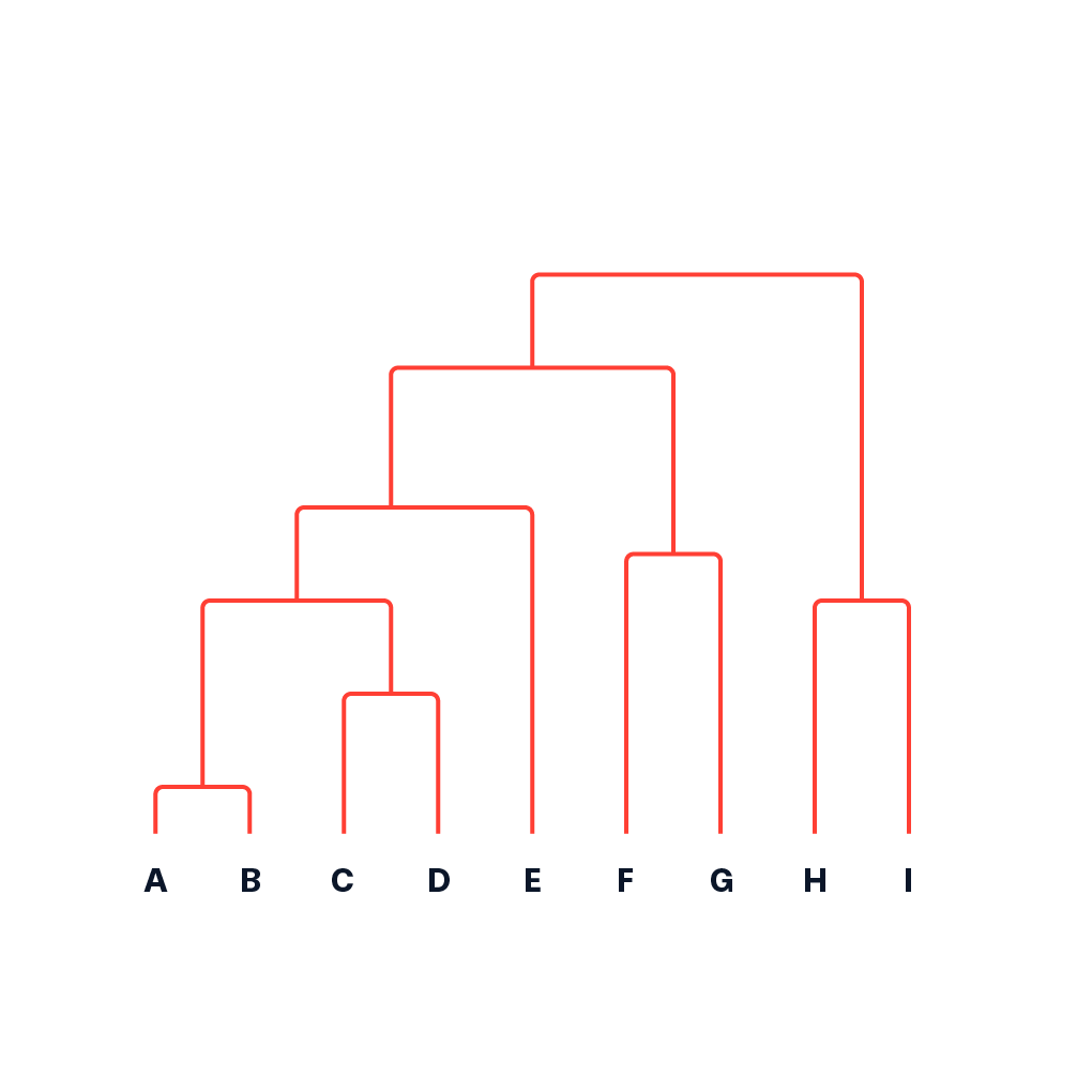
K Means

(0) Start with K random centers (also called centroids) $\mu_{1}, \mu_{2}, …, \mu_{K}$.
(1) Assign step: find points (items) that are the closest to each center k, label these points as k.
(2) Center step: update center $\mu_{k}$ to be the center of the points labeled k.
(3) Repeat until cluster centers do not change.

Total Distortion

The objective of K means clustering is minimizing the total distortion, also called inertia, the sum of distances (usually squared Euclidean distances) from the points to their centers, or $\displaystyle\sum_{i=1}^{n} \left|x_{i} - \mu_{k\left(x_{i}\right)}\right|^{2}$, where $k\left(x_{i}\right)$ is the cluster index of the cluster closest to $x_{i}$, or $k\left(x_{i}\right) = \mathop{\mathrm{argmin}}{k} \left|x{i} - \mu_{k}\right|$.

K means initialized at a random clustering and each assign-center step is a gradient descent step for minimizing total distortion by choosing the cluster centers.

Number of Clusters

The number of clusters are usually chosen based on application requirements, since there is no optimal number of clusters.

If the number of cluster is n (each point is in a different cluster), then the total distortion is 0. This means minimizing the total distortion is not a good way to select the number of clusters.

Elbow method is sometimes use to determine the number of clusters based on the total distortion, but it is a not a clearly defined algorithm

small inertia and few clusters

Dimensionality Reduction

Dimensionality reduction finds a low dimensional representation of a high dimensional point (item) in a way that points that close to each other in the original space are close to each other in the low dimensional space.

Text and image data have a large number of features (dimensions), dimensionality reduction techniques can be used for visualization and efficient storage of these data types

PCA (Principal Component Analysis)

Principal component analysis finds the orthogonal directions that capture the highest variation, called principal components, and project the feature vectors onto the subspace generated by the principal components.

Projected Variances

Projected variance along a direction u is can be computed by $u^\top \Sigma u$, so the PCA problem is given by the constrained optimization problem $\displaystyle\max_{u} u^\top \Sigma u$ subject to $u^\top u = 1$.

A closed-form solution is $\Sigma u = \lambda u$, which means $\lambda$ is an eigenvalue of $\Sigma$ and u is an eigenvector of $\Sigma$.

A faster way to find the eigenvalue-eigenvector pair is through singular value decomposition (SVD), and it is used in sklearn.decomposition.PCA

Reconstruction

If there are m original features, and m principal components are computed, then the original item can be perfectly reconstructed, if only $k<m$ principal components are used, then the original item can be approximated.

Feature	Length	Formula	Note
Original	m	$x = \begin{bmatrix} x_{i 1} \ x_{i 2} \ … \ x_{i m} \end{bmatrix}$	-
PCA Features	k	$x’ = \begin{bmatrix} u^\top_{1} x \ u^\top_{2} x \ … \ u^\top_{k} x \end{bmatrix}$	$u_{1}, u_{2}, …$are principal components
Reconstruction	m	$x = x’{1} u{1} + x’{2} u{2} + … + x’{m} u{m}$	Equal to original x
Approximation	m	$\hat{x} = x’{1} u{1} + x’{2} u{2} + … + x’{k} u{k} \approx x$	Length m, not k

Number of Reduced Dimensions

Similar to other clustering methods, the number of dimensions K are usually chosen based on application requirements (for example, 2 or 3 for visualization).

sklearn.decomposition.PCA(k) can take in k values between 0 and 1 too, and in that case, k represents the target amount of variance that needs to be explained, k for rows, colunms 不变

Auto-Encoder
If a neural network is trained with y=x, then the hidden layer unit values can be viewed as “encoding” of x.

Auto-encoder is a non-linear dimensionality reduction method if the neural network has nonlinear activations.

Reproducibility

Pseudorandom Numbers

A random sequence can be generated by a recurrence relation, for example, $x_{t+1} = \left(a x_{t} + c\right) \mod m$.

$x_0$ is called the seed, and if a,c,m are large and unknown, then the sequence looks random.

numpy.random uses a more complicated PCG generator, but with a similar deterministic sequence that looks random

Discrete Distributions

A discrete distribution takes on finite or countably infinite number of values (for example, 0, 1, 2, …).

The distribution can be summarized in a table containing the probability that it takes on each value, for example $\mathbb{P}\left{X = a\right}, a = 0, 1, 2, …$

The probabilities should be non-negative and sum up to one.

Continuous Distributions

A continuous distribution takes on uncountably infinite number of values (for example, real numbers between 0 and 1).

The distribution can be summarized as a probability density function $f\left(x\right)$ with the property that $\mathbb{P}\left{a \leq X \leq b\right} = \displaystyle\int_{a}^{b} f\left(x\right) dx$

The density function should be non-negative and integrates to 1.

For a continuous $\mathbb{P}\left{X = x\right} = 0$ always has 0 probability of taking on any specific value.

Ex:multivariate_normal([0, 0], [[1, 2], [2, 4]], 1000)

第一个矩阵表示[x_mean,y_mean]

第二个表示$\left( \begin{bmatrix} \sigma_{X}^{2} & c_{X Y} \ c_{YX} & \sigma_{Y}^{2} \end{bmatrix} \right)$

左上角是$\sigma_{X}^{2}$

correlation=$\rho_{X Y} = \dfrac{c_{X Y}}{\sigma_{X} \sigma_{Y}} = \dfrac{2}{1 \cdot 2} = 1$

Markov Chain

Stochastic Processes

A stochastic process is a sequence of random variables.

If the sequence is finite or countably infinite, it is called a discrete-time stochastic process, and the index represent the time step, usually, 0,1,….

If the sequence is uncountably infinite, it is a continuous-time stochastic process.

Markov Chains

One special class of stochastic processes is called Markov processes, where $X_t$ only depends on $X_{t-1}$, but not $X_{t-2}, X_{t-3}, …$

Formally, the sequence $X_t$ is a (discrete-time) Markov chain, $\mathbb{P}\left{X_{t} = x | X_{1} = x_{1}, X_{2} = x_{2}, …, X_{t-1} = x_{t-1}\right}$

Transition Matrices

If the time $t$ and the state distribution $X_t$are both discrete, a Markov chain can be represented by a transition matrix.

A transition matrix is a matrix where row i column j represents the probability that $\mathbb{P}\left{X_{t} = j | X_{t-1} = i\right}$

From \ to	1	2	3
1	$\mathbb{P}\left{X_{t} = 1	X_{t-1} = 1\right}$	$\mathbb{P}\left{X_{t} = 2	X_{t-1} = 1\right}$	$\mathbb{P}\left{X_{t} = 3	X_{t-1} = 1\right}$
2	$\mathbb{P}\left{X_{t} = 1	X_{t-1} = 2\right}$	$\mathbb{P}\left{X_{t} = 2	X_{t-1} = 2\right}$	$\mathbb{P}\left{X_{t} = 3	X_{t-1} = 1\right}$
3	$\mathbb{P}\left{X_{t} = 1	X_{t-1} = 3\right}$	$\mathbb{P}\left{X_{t} = 2	X_{t-1} = 3\right}$	$\mathbb{P}\left{X_{t} = 3	X_{t-1} = 1\right}$

The rows of transition matrices should sum up to 1. The columns does not have to sum up to 1.

One simple language model is the bigram model, which estimates and simulates the distribution of the next word given the current word.

Simulation and Estimation

To simulate a Markov chain with transition matrix m starting from state x0 from 0, 1, 2, …: use x1 = numpy.random.choice(len(m), p = m[x0, :]), and x2 = numpy.random.choice(len(m), p = m[x1, :]), and so on

To estimate a Markov chain transition matrix given a sequence, one way is to use the maximum likelihood estimate: $\hat{\mathbb{P}}\left{X_{t} = j | X_{t-1} = i\right} = \dfrac{c_{i j}}{c_{i}}$, where $c_{ij}$ is the number of times i is followed by j in the sequence, and $c_i$ is the number of times i appears in the sequence.