AI复习总结

参考有很多，不一一列举，还有很多懒得找了（

Search

树搜索与图搜索

Tree Search：不设置vis数组，不考虑节点有无被遍历过

搜索树（search trees）

对于一个状态出现的次数没有限制。

通过移除一个与部分计划对应的节点（用给定的策略来选择）并用它所有的子节点代替它，我们不断地扩展expand我们的边缘。用子节点代缘上的元素,相当于丢弃一个长度为n的计划并考虑所有源于它的长度为（n+1）的计划。我们继续这一操作，直到最终将目标从边缘移除为止。

Graph Search：设置vis数组，每次出堆的时候就标记visited，每次只遍历邻接的unvisited的点

图搜索（graph search）

跟踪哪些状态已经扩展过，确保每一个节点在扩展前不在这个集合中，并且在扩展后将其加入集合里。经过这种优化的树搜索称为图搜索（graph search）

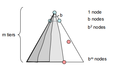
DFS(Depth-First Search)

深度优先搜索，故名意思一条边走到底再回去，优先搜索最深的边，用stack实现，头进头出

时间复杂度$O(b^m)$ 空间复杂度$O(bm)$

Complete（完备性）：定义是保证能找到答案在答案存在的情况。深度优先搜索并不具有完备性。如果在状态空间图中存在回路，这必然意味着相应搜索树的深度将是无限的。因此，存在这样一种可能性，即DFS老实地在无限大的搜索树中搜索最深的节点而不幸地陷入僵局，注定无法找到解。

Optimal：显然不是最优

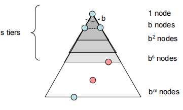
BFS(Breadth-First Search)

广度优先搜索，优先最浅的边，用queue实现，头进尾出

时间复杂度$O(b^s)$，空间复杂度$O(b^s)$，Shallowest点的深度为s

Complete：是完整的搜索

Optimal：只有cost都为1才能找到最优解

Iterative Deepening(迭代加深的深度优先搜索)

Iterative Deepening

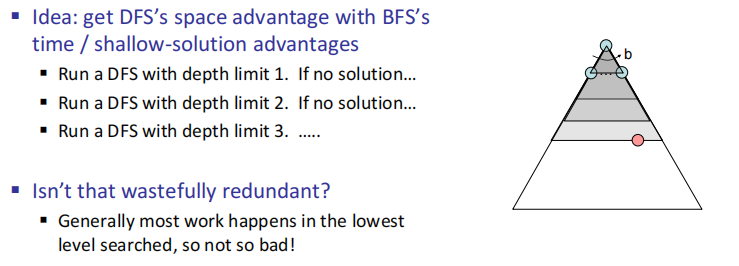
从深度为0开始，深度不断增大，直到找到目标

Complete：Yes

Optimal：Yes

时间复杂度$ O(b^d)$,空间$O(bd)$比BFS空间更优

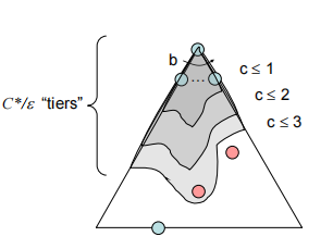
UCS(Uniform Cost Search)

优先搜索最便宜的点路径，用的是优先队列

If that solution costs $C^$ and arcs cost(两点间的最小代价) $\epsilon$ , then the“effective depth” is roughly $C^/\epsilon$

时间复杂度$O(C^*/\epsilon)$(exponential in effective depth)

空间复杂度$O(C^*/\epsilon)$

Complete：Yes

Optimal：Yes

GS(Greedy Search)

Heuristics函数，估计期望函数一般表示到重点的距离估计

贪心直往离终点最近的路走，必然不优。

Complete：Yes

Optimal：No

如果存在一个目标状态，贪婪搜索无法保证能找到它，它也不是最优的，尤其是在选择了非常糟糕的启发函数的情况下。在不同场景中。它的行为通常是不可预测的，有可能一路直奔目标状态，也有可能像一个被错误引导的DFS一样并遍历所有的错误区域。

A* Search

$f(n)=g(n)+h(n)$

结合贪心和UCS，按该点的h+该点到起点的cost

H函数的性质：①admissible：$0\leq h(n)\leq h^*(n)$，小于实际n到终点的距离。

②Consistency：$h(A)-h(C)\leq cost(A,C)$，两个点H只差小于真实距离，满足此性质即可满足最优解

Consistency $\implies$ admissibility

A* is optimal if the heuristic is admissible in the tree search.

CSP(Constraint Satisfaction Problems)

Constraint Graphs：图上相连的点表示这两个点之间有限制关系

搜索方法：

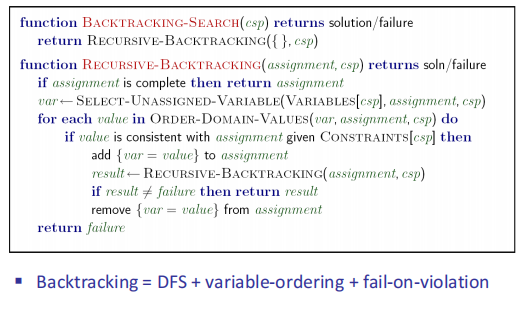
Backtracking Search：总的来说就是DFS+回溯算法，把所有可以取的值都取试一遍，可以继续就不断往下搜索，遇到问题就返回，不断撤回取值换一个值知道找到解。很慢，会走很多弯路，浪费时间。

改进过程

Filtering

每次取值的时候把不能用的过滤掉，减少取值的domain

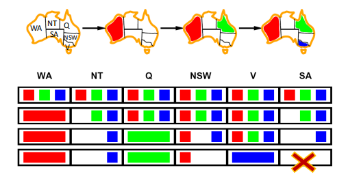
①Forward checking：每次划掉与当前取值变量有关联的变量取值，缺点是不能提前发现错误，比如在第三步的时候NT和SA都只能取蓝色其实已经矛盾了，因为每次只检查了与现在在填的格子相邻的格子取值，没有单独考虑相邻格子和其限制点的取值比较。

②Constraint Propagation：加入了每次将每个点都和其他相关的限制点domain的比较，加入consitent定义来检查每个点的限制点取值比较

An arc X → Y is consistent iff for every x in the tail there is some y in the head which could be assigned without violating a constraint

A simple form of propagation makes sure all arcs are consistent，每次propagation确保每个点都能满足consistent条件

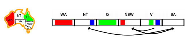
这里其实我觉得NSW也可以取蓝色，V变成红绿，这里表现能提前排除错误

K-Consistency：弧一致性是一个更广义的一致性概念——k-相容（k-consistency） 的子集，它在强制执行时能保证对于CSP中的任意k个节点，对于其中任意k-1个节点组成的子集的赋值都能保证第k个节点能至少有一个满足相容的赋值。这个想法可以通过强k-相容（strong k-consistency） 的思想进行进一步拓展。一个具有强k-相容的图拥有这样的性质，任意k个节点的集合不仅是k-相容的，也是k-1, k-2, …,1-相容的。于是，在CSP中更高阶的相容计算的代价也更高。在这一广义的相容的定义下，我们可以看出弧相容等价于2-相容。

Ordering

①最小剩余值Minimum Remaining Values (MRV)：当选择下一个要赋值的变量时，用MRV策略能选择有效剩余值最少的未赋值变量（即约束最多的变量）。这很直观，因为受到约束最多的变量也最容易耗尽所有可能的值，并且如果没有赋值的话最终会回溯，所以最好尽早赋值。

这个是针对赋值的variable的选择

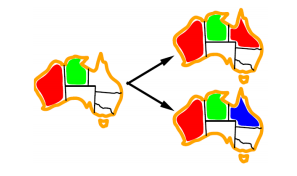
②最少约束值Least Constraining Value (LCV)：同理，当选择下一个要赋值的值时，一个好的策略就是选择从剩余未分配值的域中淘汰掉最少值的那一个。要注意的是，这要求更多的计算（比方说，对每个值重新运行弧相容/前向检测或是其他过滤方法来找到其LCV），但是取决于用途，仍然能获得更快的速度。

这个是针对对每个variable的value如何选择，尽量不要造成更多约束，选择约束最少的value，如下图应选择红色而不是蓝色

Structure

Tree-Structured CSPs

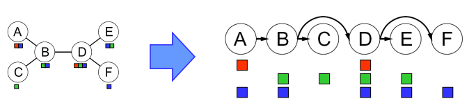
Theorem: if the constraint graph has no loops, the CSP can be solved in $O(n d^2 )$ time

首先，在CSP的约束图中任选一个节点来作为树的根节点（具体选哪一个并不重要，因为基础图论告诉我们一棵树的任一节点都可以作为根节点）。
将树中的所有无向边转换为指向根节点反方向的有向边。然后将得到的有向无环图线性化（linearize）（或拓扑排序（topologically sort））。简单来说，这也就意味着将图的节点排序，让所有边都指向右侧。注意我们选择节点A作为根节点并让所有边都指向A的反方向，这一过程的结果是如下的CSP转换：

①Remove backward: For i = n : 2, apply RemoveInconsistent(Parent(Xi ),Xi )，从孩子往父亲搜索，剪掉父亲不能consistent的值

②Assign forward: For i = 1 : n, assign Xi consistently with Parent(Xi )

从父亲开始往孩子赋值，在孩子中选取和父亲consistent的值

Nearly Tree-Structured CSPs

通过割集条件设置（cutset conditioning），树形结构算法能推广到树形结构相近的的CSP中。割集条件设置包括首先找到一个约束图中变量的最小子集，这样一来删去他们就能得到一棵树（这样的子集称为割集（cutset））。举个例子，在我们的地图染色例题中，South Australia（SA）是可能的最小的割集：

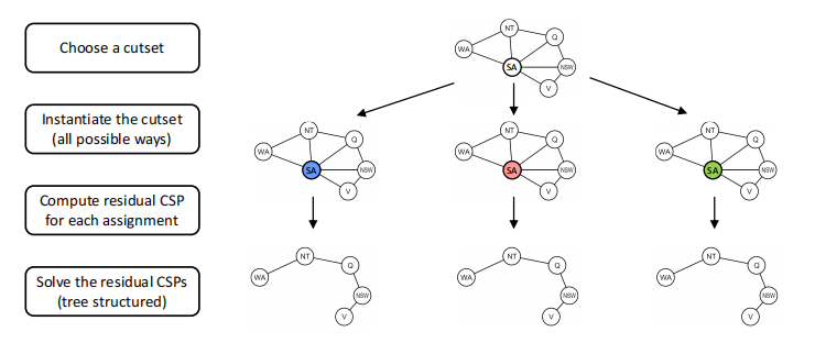
意思大概是通过不断的割掉点来减少图的边数和点数吧

Adversarial Search

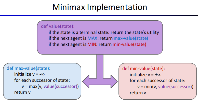
Minimax Values

基本内容就是一个人求最大，另一个人为了妨碍这个人只求最小

由于是本质还是DFS，所以复杂度是$O(b^m)$

α-β剪枝 Alpha-Beta Pruning

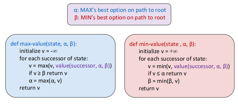
简单来说就是对于一个求最大\最小值的父亲节点的子节点，前面已经求出一个孩子的值，由于父亲只会返回最大\最下的孩子节点的值，如果某一个孩子的某一个节点已经相对于前一个孩子的值对父亲没有贡献了，就可以不搜索这个子树了，剪枝掉。

例子：下图f分支已经有b节点的10，由于a求最小，而f的100大于了10，并且e节点本身是要选最大值的，已经找出一个比较大的可能答案且比10还大，说明a节点不可能选e，故g要被剪。同理对于h节点，i这个还是是2且2已经小于了10，h本身求得的最小值已经小于a节点，根节点就不可能选h了所以l就被剪掉了。

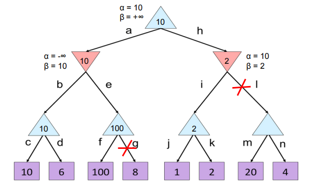
时间复杂度：$O(b^{m/2})$

讨论一下什么节点的孩子是可能会被剪掉的

①子树节点的最左边的子树一定不会被剪掉，无论如何都要比较第一个值，所以最左边最左下角的子树都要全部遍历（cd,jk)，同时所有没有被剪得节点的左边第一个孩子一定会遍历，比如上图中的f

②能被剪掉的一定是自己的siblings已经得出了部分答案，自己在被比较的过程中才会因为前一个siblings得出的答案无效所以中止检索。

估计函数 Evaluation Function

一个好的估计函数能给更好的状态赋更高的值。估计函数在深度限制（depth-limited）minimax中广泛应用，即将最大可解深度处的非叶子结点都视作叶子节点，然后用仔细挑选的估计函数给其赋虚值。由于估计函数只能用于估计非叶子结点的效益，这使得minimax的最优性不再得到保证。

$Eval(s)=w_1f_1(s)+w_2f_2(s)+ …+w_nf_n(s)$

$f(s)$ 对应从状态s中提取的一个特征，每个特征被赋予了一个相应的权重。特征就是游戏状态中能够提取并量化的一些元素。

Expectimax Search

Expectimax在游戏树中加入了机会节点（chance nodes），与考虑最坏情况的最小化节点不同，机会节点会考虑平均情况（average case）。更准确的说，最小化节点仅仅计算子节点的最小效益，而机会节点计算期望效益（expected utility） 或期望值。Expectimax给节点赋值的规则如下：

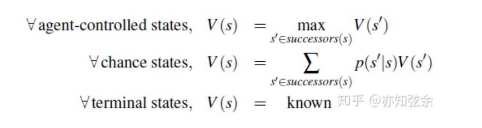
其中，$p(s’|s)$ 要么表示在不能确定操作的情况下从状态s移动到s’的概率，要么表示对手的操作使得最终从s移动到s’的概率，这取决于游戏和游戏树的特性。从这个定义来看，minimax就是expectimax的一种特例，最小化节点就是认为值最小的子节点概率为1而其他子节点概率为0的机会节点。

总的来说，概率是用来合理反映游戏状态的，但我们会在后面的笔记中更详细地介绍这一过程的原理。现在，我们可以吧这些概率看做游戏自带的特性。

Expectimax的伪代码与minimax很相似，就是把最小效益换成了期望效益，这是因为最小化节点被替换成了机会节点：

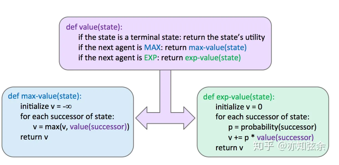
关于Expectimax，最后再说一句，需要重点注意的是，必须要遍历机会节点的所有子节点——不能再像minimax中一样进行剪枝。与minimax中求最大值或最小值时不同，每个值都会影响expectimax计算的期望值。不过，当我们已知节点有限的取值范围时，剪枝也是有可能的。

Propositional Logic

Conjunctive Normal Form (CNF)

conjunction of disjunctions of literals (clauses)

基本形式是()里面都是∪，外面套∩

Horn logic

Horn logic: only (strict) Horn clauses are allowed

– A Horn clause has the form:

$P_1 \bigcap P_2 \bigcap …P_n \implies Q$

or alternatively

$ \neg P_1 \bigcup \neg P_2 \bigcup … \neg P_n \bigcup Q$

where Ps and Q are non-negated proposition symbols

经典例题

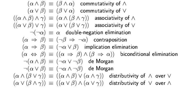
$[C \bigcup (\neg A \bigcap \neg B)] = [(\neg A \bigcap \neg B)\bigcup (C \bigcap \neg B) \bigcup ( \neg A \bigcap C) \bigcup C]$

$(\neg A \bigcup \neg B)=((A \bigcap B) \rightarrow (A \bigcap \neg A))$

Validity and satisfiability

A sentence is valid if it is true in all models

A sentence is satisfiable if it is true in some model

A sentence is unsatisfiable if it is true in no models

S is valid iff. $\neg $S is unsatisfiable

Inference

entails

$ A| !!!\ = B$ A entails B,相当于$A \implies B$

A is valid if and only if True entails A

proof

$A | !!!- B$ a demonstration of entailment from A to B

Method 1: model checking

Method 2: application of inference rules

Sound inference：everything that can be proved is in fact entailed

Complete inference：everything that is entailed can be proved

Resolution algorithm：Prove$KB |!!!= \alpha$ Proof by contradiction,show $KB |!!!= \alpha$ is unsatisfiable

把$KB \bigcap \neg \alpha$转换为CNF
. Repeatedly apply the resolution rule to add new clauses, until one of the two things happens

a) Two clauses resolve to yield the empty clause, in which

case$KB |!!! = \alpha $

b) There is no new clause that can be added, in which case

KB does not entail α

Forward chaining

从 implies 前面的条件开始往implies后面的值推导

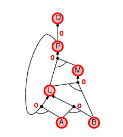
从A B L M P Q ，没往上推节点的未知数就-1，直到都为0

Backward chaining

从果找因

• Idea: work backwards from the query q:

– to prove q by BC

• check if q is known to be true already, or prove by BC all premises of some rule concluding q

• Avoid loops: check if new subgoal is already on the goal

stack

• Avoid repeated work: check if new subgoal

has already been proved true, or
has already failed

First-Order Logic

FOL

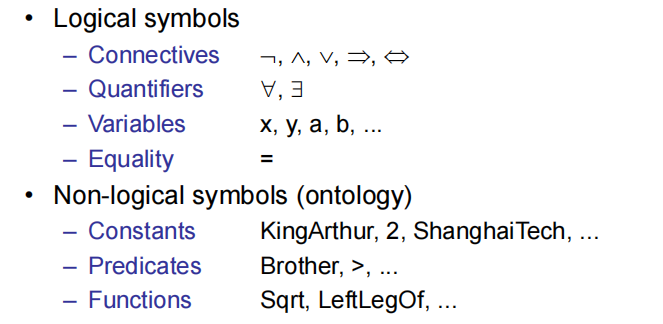
In a FOL sentence, every variable must be bound.

判断是否为FOL句式，要看变量有没有被量词限定

Atomic sentences

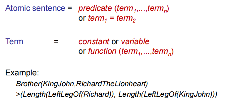
复杂句子由很多原子句子组成

任意句式：$\forall x, At(x,stu) \implies Smart(x)$(Everyone at ShanghaiTech is smart)

一般任意都接imply，不要用并

存在句式：$\exist x,At(x,stu) \bigcup Smart(x)$ (Someone at ShanghaiTech is smart)

存在句式用并，不要用imply

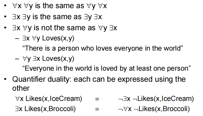
任意和存在量词的一些性质

两个变量替换原则

Universal instantiation (UI)

全称列举规则，UI 规则的实质，可以看成是包含量词的符号式的展开式，通过简化式推论规则，缩略为其中某个“合取项”。

大概是变量代入具体的意思（），变量替换

Existential Instantiation(EI)

存在列举规则

存在列举规则，就是摘除存在量词。

与 UI 不同， EI 规则摘除量词后，该行中的自由变量不是全称，而是被制定出来用以指派一个具体个体的名称。

请注意，这个个体不是被任意选出的。

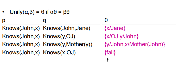
Unification

好像就是找出一个变量替换的方式。。。如下图找到x,y分别代表什么

Forward chaining

和之前那个Forward chaining差不多，从implies前的推到implies后面的

性质：

Sound and complete for first-order Horn clauses
FC terminates for first-order Horn clauses with no functions (Datalog) in finite number of iterations
In general, FC may not terminate if α is not entailed，只要没找到不会中止

Backward chaining

和之前那个Back chaining差不多，从implies后的找到implies前面的，由果及因

性质：

Depth-first recursive proof search: space is linear in size of proof线性证明
Avoid infinite loops by checking current goal against every goal on stack有效避免无限循环
Avoid repeated subgoals by caching previous results不会重复找子问题

FC and BC are sound and complete with Horn clauses and run linear in space and time.

Bayes Network

条件独立

$X \perp !!! \perp Y|Z$ : X is conditionally independent of Y given Z

$X \perp !!! \perp Y|Z \Leftrightarrow P(x|y,z)=P(x|z),P(x,y|z)=P(x|z)P(y|z)$

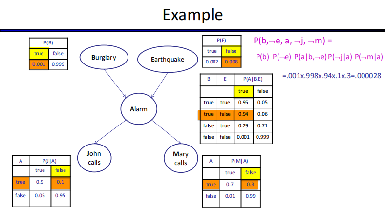
贝叶斯网络是一种描述随机变量之间互相条件独立关系的有向无环图。在这个有向无环图中，每个节点代表一个随机变量对其父节点的条件概率分布 $P(X_i|parents(X_i)$ ，每一条边可以理解成变量之间的联系。

A Bayes net = Topology (graph) + Local Conditional Probabilities

贝叶斯网络的空间：n变量，最大取值空间d，最大父节点数量k，满节点的分布$O(d^n)$贝叶斯网络大小$O(nd^{k+1})$

贝叶斯网络是有向无环图，$B \rightarrow A$ 代表B是A的条件，有公式

$P(X_1,…,X_n)=\prod_{i}P(X_i|Parents(X_i)$

When Bayes nets reflect the true causal patterns:

▪ Often simpler (fewer parents, fewer parameters)

▪ Often easier to assess probabilities

▪ Often more robust: e.g., changes in frequency of burglaries should not affect the rest of the model

BNs need not actually be causal

BN don’t need to reflect the true causal patterns

给定贝叶斯网络上部分点，判断两点是否独立：

[Step 1]. Draw the ancestral graph.

根据原始概率图，构建包括表达式中包含的变量以及这些变量的ancestor节点（父节点、父节点的父节点…）的图。注意不能包括孩子节点，不然会引起错误。

[Step 2]. “Moralize” the ancestral graph by “marrying” the parents.

连接图中每个collider结构中的父节点，即若两个节点有同一个子节点，则连接这两个节点。（若一个变量的节点有多个父节点，则分别链接每一对父节点）。

[Step 3]. “Disorient” the graph by replacing the directed edges (arrows) with undirected edges (lines).

去掉图中所有的路径方向，将directional graph变为non-directional graph。

[Step 4]. Delete the givens and their edges.

从图中删除需要判断的概率表达式中作为条件的变量，以及和他们相连的路径。比如“是否P(A|BDF) = P(A|DF)?”，我们删掉D, F变量以及他们的路径。

[Step 5]. Read the answer off the graph.

如果变量之间没有连接，则它们在给定条件下是独立的；
如果变量之间有路径连接，则它们不能保证是独立的（或者粗略地说他们是不独立的，基于概率图来说）；
如果其中一个变量或者两者都不包含在现在的图中（作为观测条件，在step 4 被删掉了），那么他们是独立的。

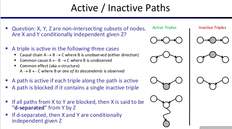
补充概念：活跃与非活跃道路

马尔可夫网络(Markov Networks)

是一个无向图

Markov network = undirected graph + potential functions

马尔可夫链

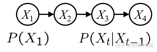
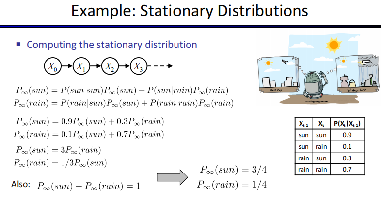
有一个特定的rule$P(X_1,X_2,…,X_t)=P(X_1)\prod_{t=2}^TP(X_t|X_{t-1})$

只需要初始概率和条件概率表（CPT）就可以得出任何一个时段，某一件事所要发生的概率。如果一个马尔可夫链接近无限长，最终概率会越来越接近一个平稳大小。

这个我们称作，静态分布（Stationary Distributions)。每一个马尔可夫链都至少有一个静态分布。对于一些特殊结构的马尔可夫链，可能只有唯一一个静态分布。比如：不可还原的（Irreducible）马尔可夫链或者叫正常的（Regular)马尔可夫链

表示的是马尔可夫链上的点可以有机会到达其它任何一个点，就表示它是Irreducible。

当一个马尔可夫链是irreducible的，那么它一定会有唯一一个静止状态。

但要想确定它是否可能最终收敛到这个静止状态，还需要另外一个属性来判断，看他是不是非周期性的（Aperiodic）

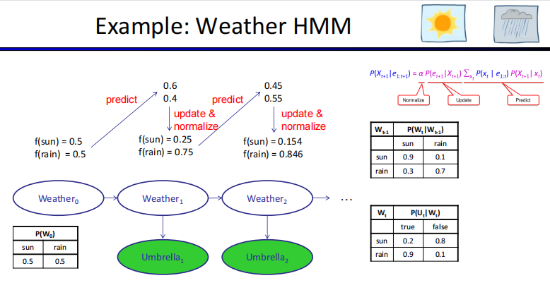
隐马尔可夫模型(HMM)

马尔可夫链的基础上加了一层可观察层，原来的链路变成了不可观察：

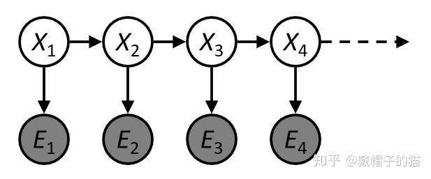
$P(X_1,E_1,…,X_T,E_T)=P(X_1)P(E_1|X_1)\prod_{t=2}^TP(X_t|X_{t-1})P(E_t|X_t)$

性质：

在已知现在(present)的可观察的状态下，未来(future)的可观察的状态，是独立于过去(past)的可观察的状态。
在已知所有的可观察的状态下，可观察的状态与可观察状态之间是独立的。

马尔可夫网络(Markov Nets)

对于马尔可夫网络中，我们也可以用势能（$\phi_i$ ）来表示不同结点间影响力的大小或者结点团之间影响力的大小。其实这个概念是源自物理中的势能。

我们可以通过一个被称作联合分布函数的来表示这个马尔可夫网络（也被称作吉布斯分布/Gibbis分布）

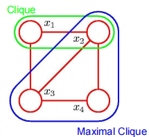
引入一个clique（小集团）的定义，用这个来定义分布

$P(X)=\frac{1}{Z}\prod_{c\in cliques(H)}\phi_c(x_c)$

$Z=\sum_x \prod_{c \in cliques(H)}\phi_c(x_c)$

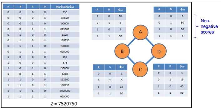
$P(X)=\frac{1}{Z}\phi_1(A,B)\phi_2(B,C)\phi_3(C,D)\phi_4(D,A)$

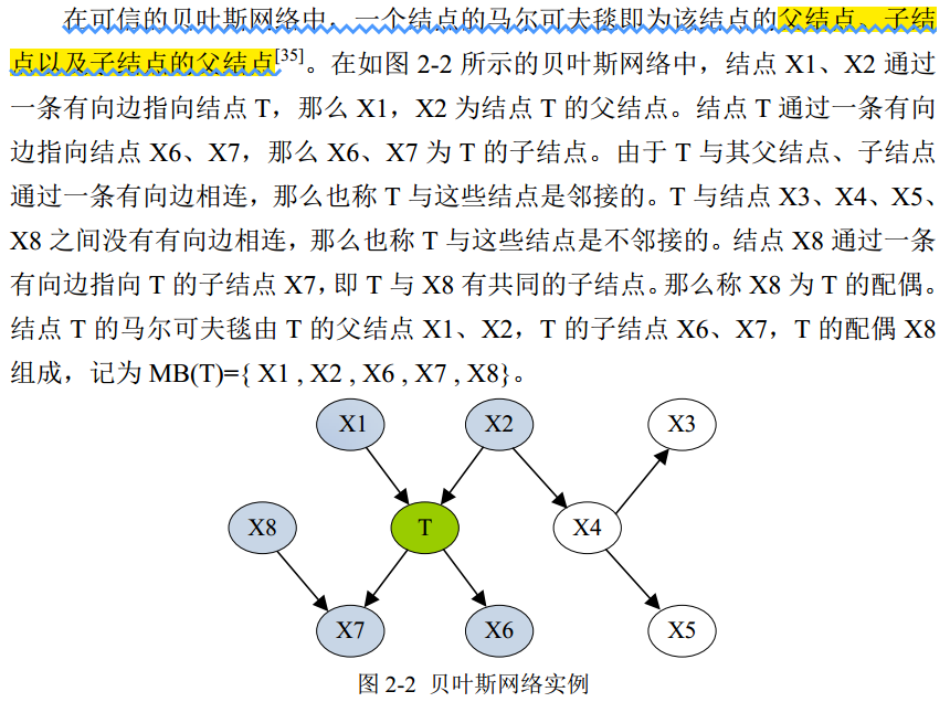
马尔可夫毯

简单来说就是T的父亲节点+T的孩子+T的孩子的父亲

贝叶斯网络和马尔可夫网络的转换

Steps

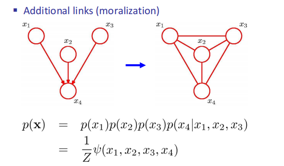
Moralization
Construct potential functions from CPTs

The BN and MN encode the same distribution，两个表示同一个分布

But they don’t encode the same set of conditional independence但表示的独立性不同

①链式结构，直接转换

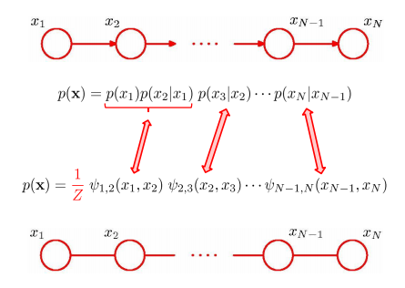
②非链式结构，要加边

只要有共同的父亲就要练边，每个父亲两两相连

Bayes Nets: Exact Inference

calculating some useful quantity from a probabilistic model (joint probability distribution)

Join factors

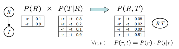
字面意思就是把条件放到条件前面去$P(r) * P(t|r) \rightarrow P(r,t)$

需要一直单独的概率和条件概率

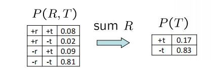
Eliminate factors

直接把某个变量删掉，必须知道联合分布

一般采用enumeration 的顺序，即从条件到非条件，沿着箭头来，但也可以不按这个顺序来。

每次eliminate一个变量就相当于把他哦才能够贝叶斯网络里面划掉，只用eliminate目标变量的祖先节点，不用管孩子节点。

Bayes Nets: Approximate Inference

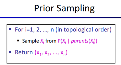
Prior Sampling (直接采样)

生成全联合概率分布，这里可以理解为路上的随机采访，因为每个节点的值概率是不一样的，所以在每个节点采样值和概率相关，我们就是通过直接采样，就像街上的直接采访一样，一个一个采样，最后生成一个概率分布表。

直接按原图的顺序一个个采就行

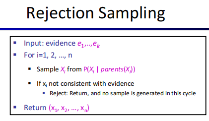
Rejection Sampling(拒绝采样)

在直接采样的基础上删去不符合的样本

对于含有随机接受度的拒绝采样，如果采样被拒绝了即取负值，则在下一个接受度重新取直到是正的再继续取别的。只要被拒绝就重新采样。

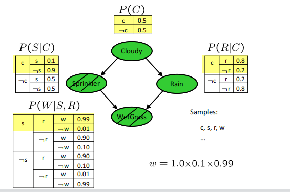
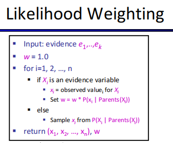
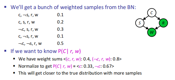
Likelihood Weighting(似然加权)

对证据变量不采样，直接利用条件分布表的概率，给每个样本一个权重，也称作似然。

我的理解就是weight就是证据变量的条件概率乘积下图的意思就是采样S,W是证据变量，其他都要有一个采样这里sample是c,s,r,w，c,r都是采样的

所以该样本weight就等于$P(S|C)P(W|S,R)$，这个1.0指的是weight一开始就是1.0给我干寂寞了之前一直没看懂

weight是evidence的$e_i,\prod_i^mP(e_i|Parents(e_i))$

下图写的就是这个过程

下面就是计算完所有权值之后再来算给定的条件概率，对比普通的采样是直接根据有多少个才看作是w，这个是每个w不同

还有一种给你随机序列让你完成一组采样和weight计算的类型

estimate$P(C=1|B=1,E=1)$，已知B,E为evidence，要采样剩余的A,C,D

采样标准：select a value $a$ from the table, and choose $W=1$if$a \geq P(W=0) $

根据第一个值0.249>0.2,A=1,0.052<0.6,C=0,0,299<0.6 D=0

故A=1,C=0,D=0

$weight=P(B|A)P(\neg C,\neg D|E)=0.8*0.8=0.64$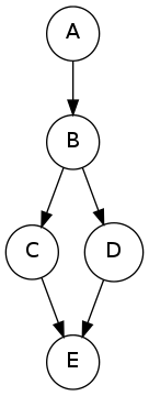

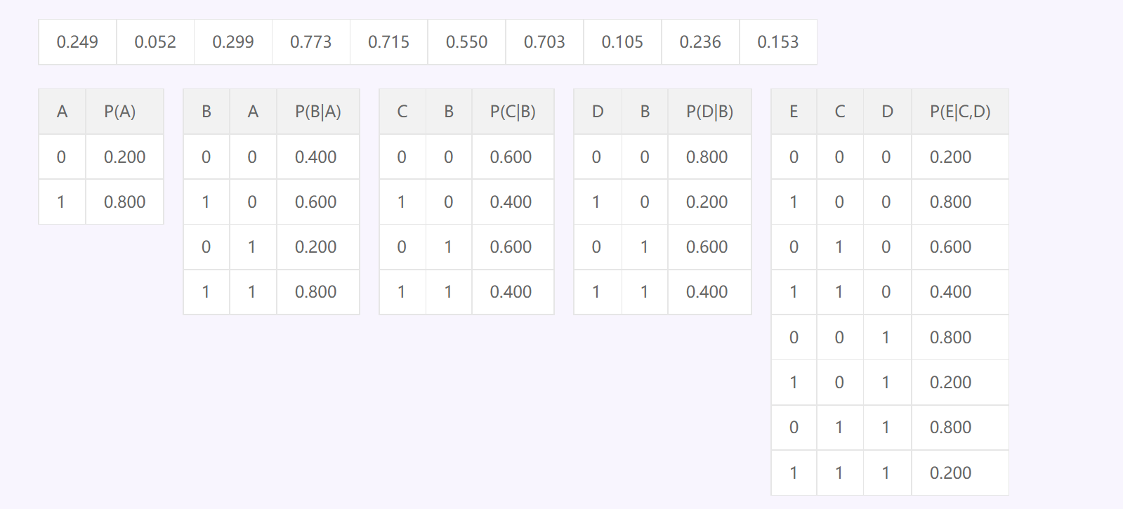
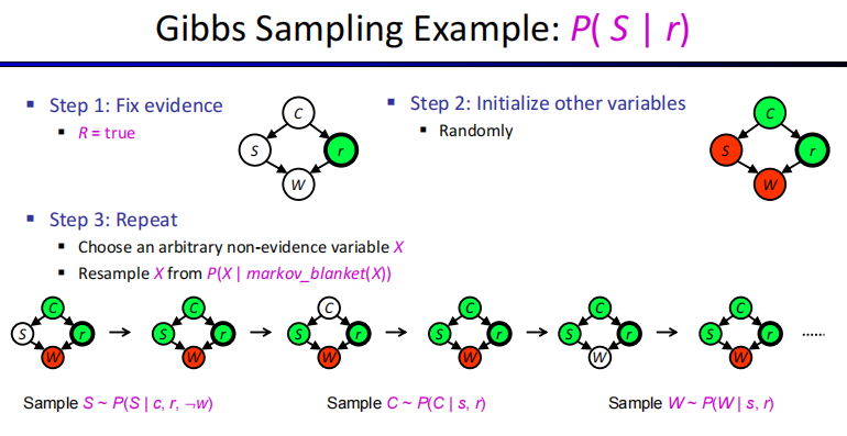
Gibbs Sampling(吉布斯采样)

先确定一个evidence，已经有一个固定值了，然后随机初始化其他的所有变量，之后随便选一个不是evidence I的变量进行采样，现要求这个I的马尔可夫毯的条件概率如下图就是

再求$p(s|c,r,\neg w)=w(s|c,r,\neg w)/(w(s|c,r,\neg w)+w(\neg s|c,r,\neg w))$

$p(\neg s|c,r,\neg w)=w(\neg s|c,r,\neg w)/(w(s|c,r,\neg w)+w(\neg s|c,r,\neg w))$

一般来说是直接算完就行了，可能会给一个接受率然后根据这个来决定sample T还是F，可能会给一个随机值r让$r \leq p(s|c,r,\neg w))$就取T，不然就是F~~~~

MCMC(Markov Chain Monte Carlo)

Markov chain = a sequence of randomly chosen states (“random walk”), where each state is chosen conditioned on the previous state

MCMC = sampling by constructing a Markov chain

基本思路：在随机变量x的状态空间S上定义一个满足遍历定理的马尔可夫链$X=x_0,x_1,…,x_t,….$，使得平稳分布就是抽样的目标分布$p(x)p ( x ) 。然后在这个马尔可夫链上开始随机游走，每个时刻得到一个样本。根据遍历定理，当时间趋于无穷时，样本的分布是趋于平稳分布的，样本的函数均值趋于函数的期望均值。所以说当时间足够长时(比如说当n>m时)(从时刻1到m我们称之为燃烧期)，在m时刻之后的时间里随机游走得到的样本值就是对目标分布抽样的结果，得到的函数均值就是近似函数的数学期望。

马尔可夫蒙特卡罗法基本步骤：

首先，在随机变量x的状态空间S上构造一个满足遍历定理的马尔科夫链，使其平稳分布为目标分布$p(x)$。
从状态空间中的某一点开始出发，用构造的马尔科夫链进行随机游走，产生样本序列$x_0,x_1,…,x_t$。
确定正整数m和n，得到样本值集合$x_{m+1},…,x_n$。求的函数$f(x)$的均值：$E_{p(x)}[f(x)]=\frac{1}{n-m}\sum_{i=m+1}^nf(x_i)$

Metropolis-Hastings

首先先定义采样时刻t-1的采样值为x，t时刻的采样值为x’，所以对于要抽样的概率分布$p(x)$采用转移核为$p(x,x’)$的马尔科夫链：$p(x,x’)=q(x,x’)\alpha(x,x’)$

其中$q(x,x’)$和$\alpha(x,x’)$分布被称之为提议分布和接受率。而提议分布是另一个马尔可夫链的转移核，是一个比较容易抽样的分布。而接受分布$\alpha(x,x’)$是：$\alpha(x,x’)=min(1,\frac{p(x’)q(x’,x)}{p(x)q(x,x’)})$

任意选一个初始值$x_0$
对于$i=1,2,…,n$ 循环操作 ①对于$x_{i-1}=x$按分布$q(x,x’)$ 随机抽取一个候选状态$x’$②计算$\alpha(x,x’)$③在(0,1)中去一个随机值如果$\alpha(x,x’)\geq u$
则$x_i=x’$否则$x_i=x$
最后得到样本合集$x_{m+1},…,x_n$，算$E_{p(x)}[f(x)]=\frac{1}{n-m}\sum_{i=m+1}^nf(x_i)$

吉布斯采样就是接受值一直为1的特例，一直接受新采样的样本

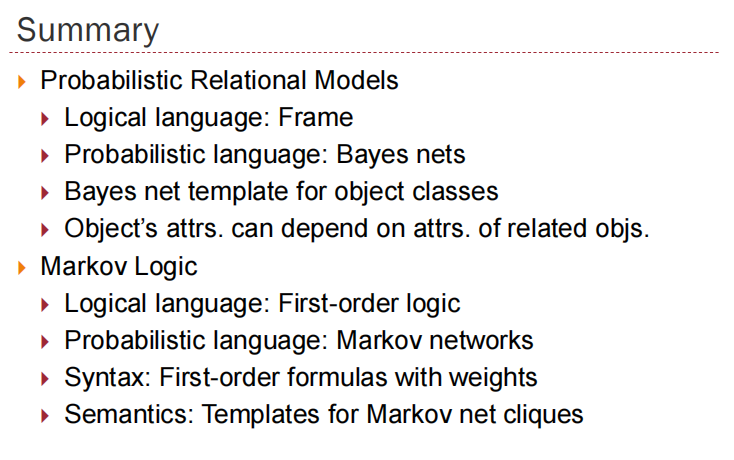
Markov logic

A Markov Logic Network (MLN) is a set of pairs (F, w)

where

F is a formula in first-order logic
w is a real number

Together with a set of constants, it defines a Markov network with

One node for each grounding of each predicate in the MLN
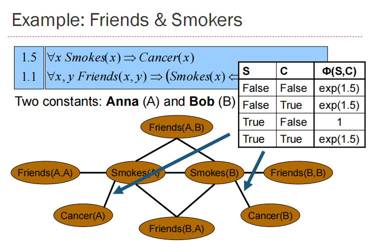
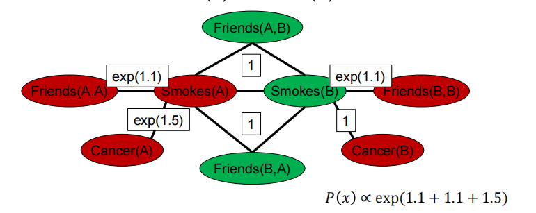
One clique for each grounding of each formula F in the MLN, with the potential being: exp(w) for node assignments that satisfy F, 1 otherwise

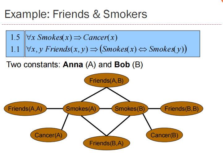
MLN is template for ground Markov nets

Probability of a word x: $P(x)=\frac{1}{Z}(\sum_iw_in_i(x))$,$w_i$ weight of formula i, $n_i(x)$ No. of true groundings of formula i in x

Infinite weights -> First-order logic

Markov logic allows contradictions between formulas

Relation to PRM

MLN is More general and flexible than PRM
In principle, a PRM can be converted into a MLN by writing a formula for each entry of each CPT and setting the weight to be the logarithm of the conditional probability

Markov Models

▪ Past and future independent given the present

▪ Each time step only depends on the previous

first-order Markov model

Stationary distribution

求无限的分布时候：$P_{\infty }(X)=\sum_xP(X|x)P_{\infty}(x) $

HMM

If the hidden state at time t is given, both the evidence at time t and the hidden state at time t + 1 are independent of the hidden state at time t − 1.

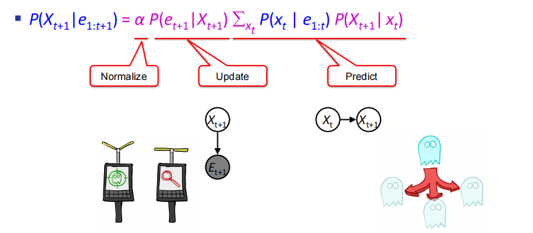
先求$P(x_t|e_{1:t})$，一般为已知，没有e0就直接用，有先算$P(x_0|e_0)=P(e_0|x_0)P(x_0)$
再求$P(e_{t+1}|x_{t+1})\sum_{x_t}P(x_t|e_{1:t})P(X_{t+1}|x_t)$
最后标准化

$P(X_{t+1}|e_{1:t})=\sum_{X_t}P(X_t|e_{1:t})P(X_{t+1}|X_t,e_{1:t})$

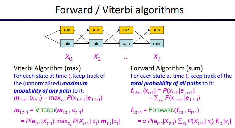
Forward algorithm

cost per time:$O(|X|^2)$,$|X|$ 是state数量

$f_{1:t+1}=\alpha P(e_{t+1}|x_{t+1})\sum_{x_t}f_{1:t}[x_t]P(X_{t+1}|x_t)$

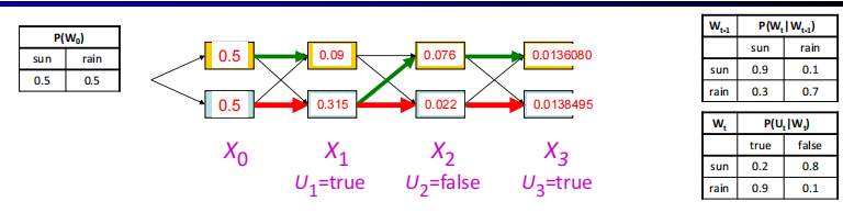
Viterbi algorithm

Forward求和，这个求最大值

$m_{1:t+1}=P(e_{t+1}|x_{t+1})max_{x_t}{m_{1:t}[x_t]P(X_{t+1}|x_t)}$

Time:$O(|X|^2T)$, Space $O(|X|T)$,T length of sequence

Both the time complexity and the space complexity of the Viterbi algorithm are linear in the length of the sequence.

两者比较，时间复杂度相同

Dynamic Bayes Nets

▪ Every HMM is a DBN，hmm都是dbn

Every hidden Markov model can be represented as a dynamic Bayesian network with a single state variable and a single evidence variable.

▪ Each HMM state is Cartesian product of DBN state variables

▪ Every discrete DBN can be represented by a HMM，只有离散的dbn才是hmm

DBN优点：参数更少，Sparse dependencies

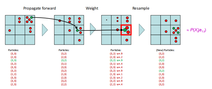
Particle Filtering

Represent belief state at each step by a set of samples（Samples are called particles）

Each iteration of particle fifiltering consists of propagate forward, observe and resample

Initialization

▪ sample N particles from the initial distribution $P(X_0 ）$，All particles have a weight of 1

▪ Each particle is moved by sampling its next position from the transition model:$x_{t+1} $~$P(X_{t+1}|x_t)$

▪ Similar to likelihood weighting, weight samples based on the evidence $W=P(e_t|x_t)$

▪ Rather than tracking weighted samples, we resample. Each new sample is selected from the current population of samples; the probability is proportional to its weight

Markov Decision Processes

MDPs are non-deterministic search problems

MDP satisfy the memoryless property.

马尔可夫决策过程是一个五元组，求解一个马尔可夫决策过程，则意味着找到最优策略π*

S：有限状态集

A：有限动作集

P：状态转移矩阵 (也有的地方是T)

R：奖励函数

γ：折扣因子是给定状态的动作分布 状态值函数：
动作值函数： 状态值函数的贝尔曼期望方程：某一个状态的价值可以用该状态下所有动作的价值表述动作值函数的贝尔曼期望方程：某一个动作的价值可以用该状态后继状态的价值表述，及发生了动作a的价值

贝尔曼(Bellman)方程

一个状态s的最优值$V^*(s)$

——s的最优值是一个从s出发的agent在其余下寿命中采取最优行动能获得的效益的期望值。

一个q状态(s,a)的最优值$Q^*(s,a)$

——(s,a)的最优值是一个agent从状态s采取行动a之后获得的效益的期望值，并且该agent从此以后采取的都是最优行动。

最优策略$\pi ^*(s)$

$Q^(s,a)=\sum_{s’}T(s,a,s’)[R(s,a,s’)+ \gamma V^(s’)]$,$V^(s)=max_a\sum_{s’}T(s,a,s’)[R(s,a,s’)+\gamma V^(s’)]$

值迭代 (Value Iteration)求解马尔科夫决策过程

现在我们有了一个能验证MDP中各状态的值的最优性的框架，接下来自然就想知道如何能精确计算出这些最优值。为此我们需要限时值（time-limited values）（强化有限界得到的结果）。限制时间步数为k的一个状态s的限时值表示为 $V_k(s)$ ，代表着在已知当前MDP会在k时间步后终止的情况下，从s出发能得到的最大期望效益。这也正是一个在MDP的搜索树上执行的k层expectimax所返回的东西。

简单来说，值迭代就是给定k，也就是步数为k，在这k步之内，我们希望值迭代已经到达稳定状态，即下一次迭代与这一次的完全相同，这时我们就得到一个最优决策，也就是从哪里出发能够得到最大期望效益。

$V_{k+1}(s)\leftarrow max_a \sum_{s’}T(s,a,s’)[R(s,a,s’)+\gamma V_k(s’)]$

Time:$O(S^2A)$

$V_k$ converge as long as $\gamma <1$

策略迭代 Policy Iteration求解马尔科夫决策过程

Time:$O(S^2A)$

策略提取 Policy Extraction

还记得我们解决MDP的最终目标是要确定一个最优策略。只需要确定所有状态的最优值就能达成这一目标，这可以通过一种叫策略提取(policy extraction)的方法来实现。策略提取的背后的思想非常简单：如果你处于一种状态s，你应该采取会产生最大期望效益的行动a。不难想到，a正是会将我们带到具有最大q值的q状态的操作，于是最优策略可以表达为：

$\pi^(s)=argmax_a\sum_{s’}T(s,a,s’)[R(s,a,s’)+\gamma V^(s’)]$

为了取得最好的效益，状态的最优q值对策略提取来说是最好的，因为在这种情况下，只需要一次argmax就能确定从一个状态出发的最优行动。仅保存每个 $V^*(s)$意味着我们必须在取argmax之前用Bellman方程重新计算所有必须的q值，相当于进行一次深度为1的expectimax。

策略迭代 Policy Iteration

值迭代可能会很慢。在每次迭代中，我们必须更新所有|S|个状态的值（|n|表示集合中元素的个数），其中每个都要求在我们计算每个行动的q值时对所有|A|个行动进行迭代。对这些每个q值的计算，需要轮流对|S|个状态再次进行迭代，导致时间成本过高。此外，当我们只想确定MDP的最优策略时，值迭代会进行大量多余的计算，因为由策略提取得到的策略通常会比值本身更快地收敛。修正这些缺陷的方法就是选择策略迭代，这种算法可以在保持值迭代的最优性的同时还能对表现进行大幅提升。策略迭代的操作如下：

定义一个初始策略。这个可以随意定，但是如果初始策略越接近最优策略，策略迭代收敛得也就越快。
重复以下操作，直至收敛：
用策略评估对当前策略进行评估。对于一个策略π，策略评估意味着计算所有状态s的Vπ(s)，其中Vπ(s)表示按照策略π从状态s出发的期望效益： $V^\pi (s)=max_a\sum_{s’}T(s,a,s’)[R(s,a,s’)+\gamma V^\pi(s’)]$
把策略迭代的第i次迭代成为πi。由于我们正在对每个状态的一个行动进行修正，我们不再需要取最大的操作max operator，这样我们得到的系统就能有效由以上规则生成的|S|个方程构成的。然后每个$V^{\pi_i}(s)$ 就可以通过解决这个系统来计算得到。

评估完当前策略后，用策略改进 policy improvement来生成更好的策略。策略改进通过对由策略评估生成的状态的值进行策略提取，生成以下改进提升后的策略：

$\pi_{i+1}(s)=argmax_a\sum_{s’}T(s,a,s’)[R(s,a,s’)+\gamma V^{\pi_i}(s’)]$

策略迭代就是给定初始策略，不断进行策略评估->策略提取->策略改进直至收敛

值迭代和策略迭代比较

▪ Both value iteration and policy iteration compute the same thing (all optimal values)计算一样的东西

▪In value iteration:

▪ Every iteration updates both the values and (implicitly) the policy

▪ We don’t track the policy, but taking the max over actions implicitly recomputes it

▪ In policy iteration:

▪ We do several passes that update utilities with fixed policy (each pass is fast because we consider only one action, not all of them)

▪ After the policy is evaluated, a new policy is chosen (slow like a value iteration pass)

▪ May converge faster，会更快收敛

Both are dynamic programs for solving MDPs

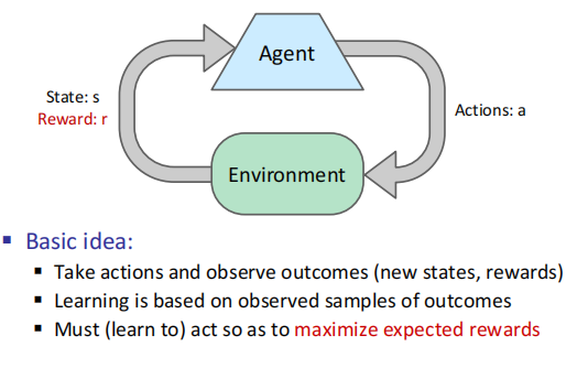
Reinforcement Learning

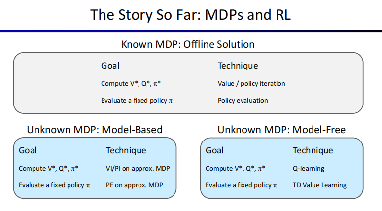
Offline Planning

▪ You determine all quantities through computation

▪ You need to know the details of the MDP

▪ You do not actually play the game!

Online Planning

不需要transition model for states and actions，reward funcition for every allowed transition between states

Model-Based Learning

离线学习(off-line)也通常称为批学习，是指对独立数据进行训练，将训练所得的模型用于预测任务中。将全部数据放入模型中进行计算，一旦出现需要变更的部分，只能通过再训练(retraining)的方式，这将花费更长的时间，并且将数据全部存在服务器或者终端上非常占地方，对内存要求高。Q学习就是离线学习

在线学习(in-line)也称为增量学习或适应性学习，是指对一定顺序下接收数据，每接收一个数据，模型会对它进行预测并对当前模型进行更新，然后处理下一个数据。这对模型的选择是一个完全不同，更复杂的问题。需要混合假设更新和对每轮新到达示例的假设评估。换句话说，你只能访问之前的数据，来回答当前的问题。

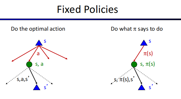
Model-Free Learning

Input: a fixed policy (s)
You don’t know the transitions T(s,a,s’)
You don’t know the rewards R(s,a,s’)
Goal: learn the state values

Direct Evaluation

Goal: Compute values for each state under $\pi$

Idea: Average together observed sample values

▪ Act according to $\pi$

▪ Every time you visit a state, write down what the sum of discounted rewards turned out to be

▪ Average those samples

Good:

▪ It’s easy to understand

▪ It doesn’t require any knowledge of T, R

▪ It eventually computes the correct average values, using just sample transitions

Bad:
▪ It wastes information about state connections

▪ Each state must be learned separately

▪ So, it takes a long time to learn

Passive Reinforcement Learning

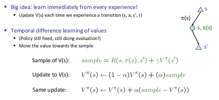
TD学习的基本思想是从每一次经验中学习（这里我的理解是从v中学习，一定程度上也可以称为v学习），而不是像直接评估那样简单地记录总奖励和访问状态并在最后学习。在策略评估中，我们使用固定策略和贝尔曼方程产生的方程评估该策略下的状态值：

Temporal Difference Learning

▪ (Policy still fixed, still doing evaluation!)

▪ Move the value towards the sample

Decreasing learning rate (alpha) can give converging averages

Model-Based Learning

▪ Learn an approximate model based on experiences

▪ Solve for values as if the learned model was correct

Step 1: Learn empirical MDP model
Step 2: Solve the learned MDP

Active Reinforcement Learning

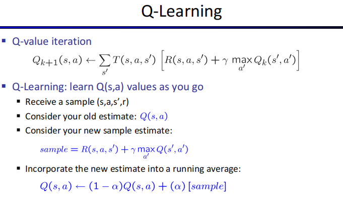
Q-learning can converge to the optimal policy even if you are acting sub-optimally when you explore.

The factor for Q-learning to converge to the optimal Q-values:

Every state-action pair is visited infinitely often.
The learning rate is decreased to 0 over time.

Full reinforcement learning

▪ You don’t know the transitions T(s,a,s’)

▪ You don’t know the rewards R(s,a,s’)

▪ You choose the actions now

▪ Goal: learn the optimal policy / values

Q-learning：off-policy learning

Regret

The $\epsilon $-greedy strategy often produces a lower regret for a decaying $\epsilon$ than a fixed one.

Regret is a measure of your total mistake cost: the difference between your (expected) rewards, including youthful suboptimality, and optimal (expected) rewards

Minimizing regret goes beyond learning to be optimal – it requires optimally learning to be optimal

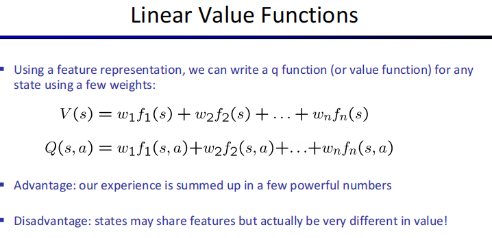
Approximate Q-Learning

Approximate Q-learning is model-free learning

▪ Learn about some small number of training states from experience

▪ Generalize that experience to new, similar situations

Compared with Q-learning, approximate Q-learning that describes each state with a vector of features can be helpful when the number of states is huge.

Linear Value Functions

Q-learning:

transition=$(s,a,r,s’)$

difference=$[r+\gamma max_{a’}Q(s’,a’)]-Q(s,a)$

$Q(s,a)=Q(s,a)+\alpha [difference],w_i=w_i+\alpha [difference]f_i(s,a)$

Supervised Machine Learning

Naïve Bayes

$P(Y,F_1,…,F_n)=P(Y)\prod _iP(F_i|Y)$

nx|F|x|Y| parameters

Total number of parameters is linear in n

Goal: compute posterior distribution over label variable

The na ̈ıve Bayes assumption takes all features to be independent given the class label.

Overfitting过拟合

原因：

1.训练集的数据太少

2.训练集和新数据的特征分布不一致

3.训练集中存在噪音。噪音大到模型过分记住了噪音的特征，反而忽略了真实的输入输出间的关系。

4.权值学习迭代次数足够多，拟合了训练数据中的噪音和训练样例中没有代表性的特征。

解决方法：

加大数据集（Training and test Set）使模型在训练的过程中尽可能多的见到更多的问题，从而使学到的分布更加全面更加General。比如采集更多的样本，或者采取Data Augmentation的方法。

改进你的模型。
2.1. 比如将你的模型进行简化，从而减少一些不重要的参数和属性。比如如果你使用神经网络，你可以减少Hidden Layer，或者减少每个Hidden Layer中的神经元数量（Dropout等）；或者如果你使用Adaboost这类的Ensemble Learning方法，你可以减少模型所包含的Weak Learner的数量，并且尽可能的简化每一个Weak Learner。
2.2 你也可以采取一些Regularization的方法主动地调节模型的参数值，比如L1， L2 Norm等等。采用这类方法，可以很大程度的惩罚模型内部的参数，从而阻止Overfitting的发生。（之后的专栏会有介绍）。

提前结束无意义的训练 Early Stop。比如当我们训练一个Logistic Regression时，我们的目标是专注于找到合适的参数，使Loss（error）尽可能的小。如果重复过多次数的训练，会导致训练出来的模型过分专注于解决训练集，从而使模型不具备Generalization。如下图，可以看到，过多的training iteration，确实可以降低Training Loss，但是也会使模型过分专注于training Samples,从而使Test Loss提高（即Overfit）。这时候我们需要提前结束训练，阻止Test Error的提升。

Avoid overfitting

Acquire more training data (not always possible)
Remove irrelevant attributes (not always possible)
Limit the model expressiveness by regularization, early stopping, pruning, etc.
We can use smoothing or regularization to improve model’s generalization.

we may smooth the empirical rate to improve generalization

Laplace Smoothing

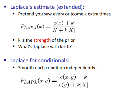
$c(x)$权重，k给定，|X|x有多少取值，N x权重和

Linear Regression

Least squares: Minimizing squared error最小二乘法

Unsupervised Machine Learning

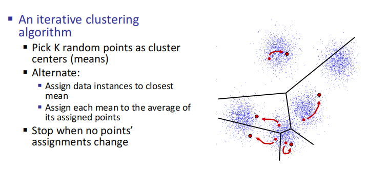
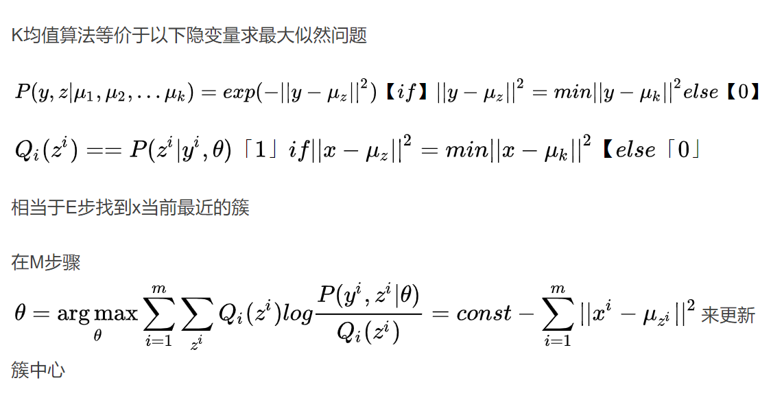
K-Means

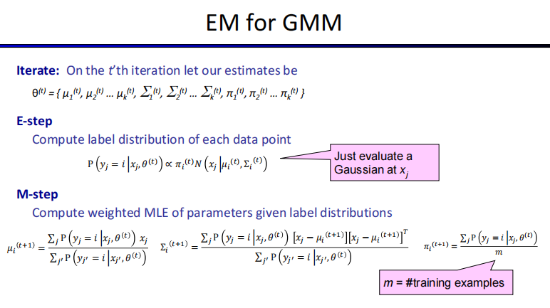
EM

The EM algorithm can be used to learn any model with hidden variables (missing data)

[E step] Compute probability of each instance having each possible label，Compute label distribution of each data point

[M step] Treating each instance as fractionally having both labels,

compute the new parameter values，Compute weighted MLE of parameters given label distributions, When using the EM algorithm to learn a Gaussian mixture model, the M-step computes weighted maximum likelihood estimation (MLE).

The label distributions computed at E-step are point-estimations

EM & K-means

A neural network with a sufficient number of neurons and a complex enough architecture can approximate any continuous function to any desired accuracy.

In Convolutional Neural Networks, different hidden units organized into the same “feature map” share weight parameters.

Natural Language Processing

Context-Free Grammars

four components

 A set of terminals (words)

 A set N of nonterminals (phrases)

 A start symbol SN

 A set R of production rules

 Specifies how a nonterminal can produce a string of terminals and/or nonterminals

Any arbitrary CFG can be rewritten into the Chomsky normal form (CNF), Probabilistic CFGs tend to assign larger probabilities to smaller parse trees.

CFG(Chomsky Normal Form)，乔姆斯基规范形式

具有以下形式：

A -> a
A -> BC
S -> ε

小写字母表示终结符号，大写表示非终结符。
产生式的体要么由单个终结符号或者ε构成，要么由两个非终结符构成。

题目转换只需要满足箭头后面只有两个大写单词，不会是一个或者三个，多于两个用x新增一行，只有一个向下面合并

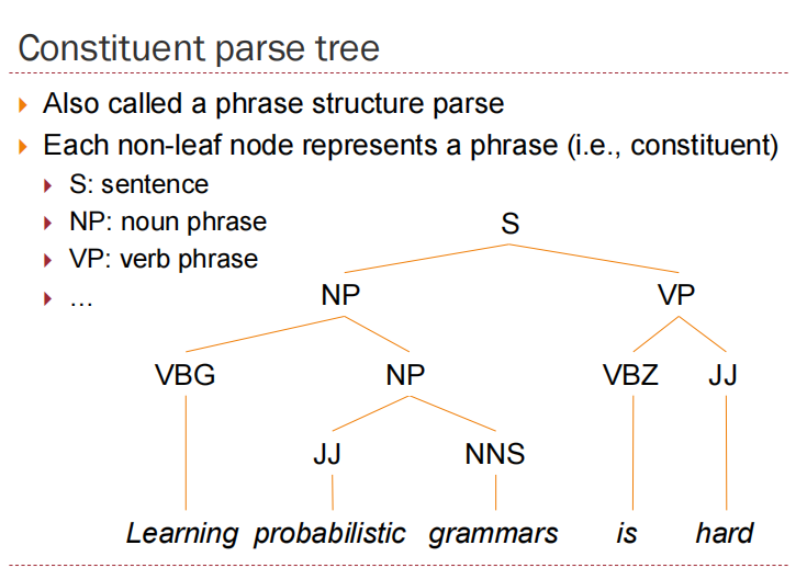
Ambiguity: A sentence is ambiguous if it has more than one possible parse tree

Probabilistic CFGs have ambiguity problem.

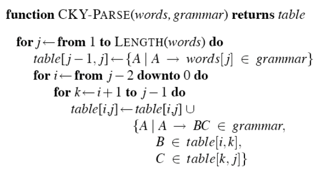
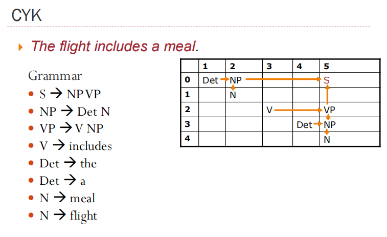
Cocke–Younger–Kasami Algorithm (CYK)

Base case:

 A is in cell [i-1,i] iff. there exists a rule A → wi

Recursion:

 A is in cell [i,j] iff. for some rule A → B C there is a B in ell [i,k] and a C in cell [k,j] for some k.

图示

Dependency Parse

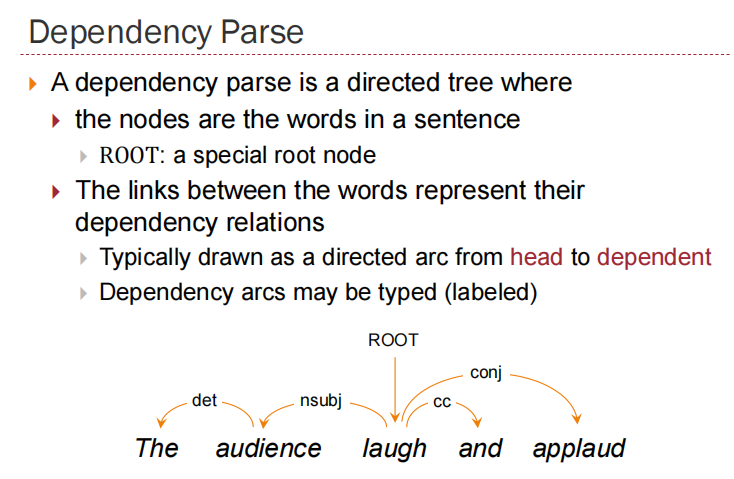
The links between the words represent their dependency relations

Dependency parses of sentences having the same meaning are more similar across languages than constituency parses

Parsing can be faster than CFG-bases parsers

Graph-based parsing

Parsing: find the highest-scoring parse tree

Taking a string and a grammar and returning one or more parse tree(s) for that string